Here is a term paper on the ‘Indifference Curve Analysis’ for class 9, 10, 11 and 12. Find paragraphs, long and short term papers on the ‘Indifference Curve Analysis’ especially written for commerce students.
Term Paper on Indifference Curve Analysis
Term Paper Contents:
- Term Paper on Indifference Curve Approach
- Term Paper on What are Indifference Curves?
- Term Paper on the Properties of Indifference Curves
- Term Paper on the Indifference Curves of Perfect Substitutes and Perfect Complements
- Term Paper on Consumer’s Equilibrium: Maximising Satisfaction
- Term Paper on the three Demand Theorems Based on Indifference Curve Analysis
- Term Paper on the Derivation of Individual’s Demand Curve from Indifference Curve Analysis
- Term Paper on the Superiority of Indifference Curve Analysis
- Term Paper on Is Indifference Curve Analysis “The Old Wine in a New Bottle”?
- Term Paper on the Critique of Indifference Curve Analysis
A popular alternative theory of consumer’s demand is the Indifference Curve Analysis which forms the subject-matter of the present article. The technique of indifference curves was first of all invented by a classical economist Edgeworth but he used it only to show the possibilities of exchange between two persons and not to explain consumer’s demand.
ADVERTISEMENTS:
Two English economists, J.R. Hicks and R.G D. Allen in their now well-known paper ‘A Reconsideration of the Theory of Value’ severely criticised Marshall’s utility analysis based upon cardinal measurement of utility and put forward the indifference curve approach based upon the notion of ordinal utility to explain consumer’s behaviour. In 1939 Hicks reproduced the indifference curve theory of consumer’s demand in his book “Value and Capital’ modifying somewhat the version of the original paper.
Term Paper # 1. Indifference Curve Approach:
Indifference curve method has been evolved to supersede the marginal utility analysis of demand. The indifference curve method seeks to derive all rules and laws about consumer’s demand that are derivable from the cardinal utility analysis. At the same time the inventors and supporters of new method contend that their analysis is based on fewer and more reasonable assumptions.
The indifference curve analysis has, however, retained some of the assumptions of Marshall’s cardinal utility analysis. Thus, the indifference curve approach, like the old cardinal utility approach, assumes that the consumer possesses ‘complete information’ about all the relevant aspects of economic environment in which he finds himself. For example, the prices of goods, the markets in which they are available, the satisfaction to be obtained from them etc., are all known to the consumer.
Further, it is assumed that the consumer acts rationally in the sense that, given the prices of goods and the money income, he will choose the combination from among the various possible combinations that gives him maximum satisfaction. Moreover, the assumption of ‘continuity’ has also been retained by Hicks-Allen indifference curve method. Continuity assumption means that the consumers are capable of ordering or ranking all conceivable combinations of goods according to the satisfaction they yield.
ADVERTISEMENTS:
The fundamental approach of indifference curve analysis is that it has abandoned the concept of cardinal utility and instead has adopted the concept of ordinal utility. According to the supporters of the indifference curves theory, utility is a psychic entity and it cannot therefore be measured in quantitative cardinal terms. In other words, utility being a psychological feeling is not quantifiable.
The concept of cardinal utility, according to the exponents of the indifference curve theory, is therefore untenable. On the other hand, the assumption of ordinal utility, according to them, is quite reasonable and realistic. The ordinal utility implies that the consumer is capable of simply ‘comparing the different levels of satisfaction’.
In other words, according to the ordinal utility hypothesis, while the consumer may not be able to indicate the exact amounts of utilities that he derives from commodities or any combination of them, but he is capable of judging whether the satisfaction obtained from a good or a combination of goods is equal to, lower than, or higher than another.
For deriving the theory of consumer’s behaviour, it is sufficient to assume that the consumer is able to rank his preferences consistently. Thus, the basis of indifference curve analysis of demand is the preference-indifference hypothesis. This means that if the consumer is presented with a number of various combinations of goods, he can order or rank them in ‘scale of preferences’.
ADVERTISEMENTS:
If the various combinations are marked A, B, C, D, E, etc. the consumer can tell whether he prefers A to B, or B to A, or is indifferent between them. Similarly, he can indicate his preference or indifference between any other pair of combinations. The concept of ordinal utility implies that the consumer cannot go beyond stating his preference or indifference. In other words, if a consumer happens to prefer A to B, he cannot tell by how much he prefers A to B.
Thus, under ordinal utility hypothesis, the consumer cannot tell the ‘quantitative differences’ between various levels of satisfaction; he can simply compare them ‘qualitatively’, that is, he can merely judge whether one level of satisfaction is higher than, lower than or equal to another.
Further, according to the supporters of indifference-curve method, by ‘how much’ one combination of goods is preferred to another is not even needed for deriving laws concerning consumer’s behaviour. It is sufficient to assume that the consumer is able to tell whether one combination of goods gives him greater, equal, or less satisfaction than another.
It may be noted that the consumer formulates his scale of preferences independently of the market prices of goods keeping in view only the satisfaction which he hopes to get from various combinations of goods. In consumer’s scale of preferences some combinations will occupy the same place, i.e., the consumer will be indifferent among them. Combinations occupying a higher place in the scale will be preferred to the combinations occupying lower places in the scale.
Moreover, the indifference curve analysis assumes that the preference and indifference relations are ‘transitive’. The transitivity of preference or indifference relations means that if the consumer prefers A to B, and B to C, then he will also prefer A to C and likewise, if he is indifferent between A and B, and between B and C, then he will also be indifferent between A and C.
Term Paper # 2. What are Indifference Curves?
The basic tool of Hicks-Allen ordinal analysis of demand is the indifference curve which represents all those combinations of goods which give same satisfaction to the consumer. Since all the combinations on an indifference curve give equal satisfaction to the consumer, he will be indifferent between them, that is, it will not matter to him which one he gets. In other words, all combinations of the goods lying on a consumer’s indifference curve are equally desirable to or equally preferred by him.
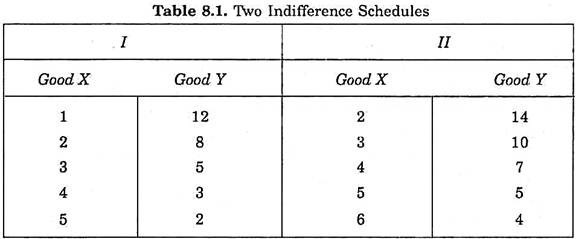
To understand indifference curves, it is better to start with indifference schedules. In Table 8.1, two indifference schedules are given. In each schedule the amounts of goods X and Y in each combination are so much that the consumer is indifferent among the combinations in each schedule. In schedule 1, the consumer has to start with 1 unit of X and 12 units of Y.
Now, the consumer is asked to tell how much of good Y he will be willing to give up for the gain of an additional unit of X so that his level of satisfaction remains the same. If the gain of one unit of X compensates him fully for the loss of 4 units of Y, then the next combination of 2 units of X and 8 units of Y(2X + 8Y) will give him as much satisfaction as the initial combination (1X + 12Y).
Similarly, by asking the consumer further how much of Y he will be prepared to forgo for successive increments in his stock of X so that his level of satisfaction remains unaltered, we get combinations 3X + 5Y, 4X + 3Y, and 5X + 2Y, each of which provides same satisfaction as combination 1X + 12Y or 2X + 8Y. Since his satisfaction is the same whichever combination of goods in the schedule is offered to him, he will be indifferent among the combinations of two goods included in the schedule.
In schedule II, the consumer has initially 2 units of X and 14 units of Y. By asking the consumer how much of Y he will be prepared to abandon for the successive additions of X in his stock so that his satisfaction remains equal to what he derives from the initial combination (2X + 14Y), we get combinations 3X + 10Y, 4X + 7Y, 5X + SY and 6X + 4Y. Thus, each of the combinations in schedule II will be equally desirable to the consumer and he will be indifferent among them. But it should be borne in mind that the consumer will prefer any combination in schedule II to any combination in schedule I.
That is, any combination in schedule II will give him more satisfaction than any combination in schedule I. This is because it is assumed that more of a commodity is preferable to less of it (in other words, the greater quantity of a good gives an individual more satisfaction than the smaller quantity of it). Initial combination in schedule II contains more of both the goods than the initial combination in schedule I, therefore the former will give greater satisfaction to the consumer than the latter.
Now, since each of the other combinations in indifference schedule II provides the same satisfaction as the initial combination (2X + 14Y) of the schedule and also each of other combinations in indifference schedule I gives the same satisfaction as the initial combination (1X + 12Y), any combination of the schedule II will be preferred to (will yield greater satisfaction than) any combination of schedule I.
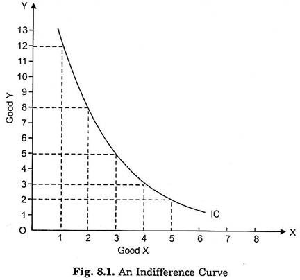
Now, we can convert the indifference schedules into indifference curves by plotting the various combinations on a graph paper. In Fig. 8.1 an indifference curve IC is drawn by plotting the various combinations of the indifference schedule I. The quantity of good X is measured on the horizontal axis, and the quantity of the good Y is measured on the vertical axis.
ADVERTISEMENTS:
As in an indifference schedule, combinations lying on an indifference curve will also be equally desirable to the consumer, that is, will give him the same satisfaction. The smoothness and continuity of an indifference curve means that goods in question are assumed to be perfectly divisible. If the indifference schedule II is also converted into indifference curve, this will lie above the indifference curve IC.
Any combination on a higher indifference curve will be preferred to any combination on a lower indifference curve. It is thus clear that the indifference curve lying above and to the right of an indifference curve will indicate higher level of satisfaction than the latter. It may be noted that while an indifference curve shows all those combinations of two goods which provide equal satisfaction to the consumer, it does not indicate exactly how much satisfaction is derived by the consumer from those combinations. This is because the concept of ordinal utility does not involve the quantitative measurability of utility. Therefore, no attempt is made to label an indifference curve by the quantity or amount of satisfaction it represents.
A complete description of consumer’s tastes and preferences can be represented by an indifference map which consists of a set of indifference curves. Because the field in a two-dimensional diagram contains an infinite number of points each representing a combination of goods X and Y, there will be an infinite number of the indifference curves each passing through combinations of goods that are equally desirable to the consumer.
ADVERTISEMENTS:
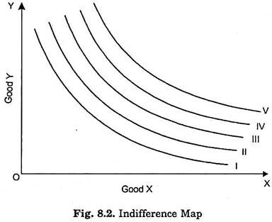
In Fig. 8.2 an indifference map of a consumer is shown which consists of five indifference curves. The consumer regards all combinations on the indifference curve I as giving him equal satisfactions. Similarly, all the combinations lying on indifference curve II provide the same satisfaction but the level of satisfaction on indifference curve II, will be greater than the level of satisfaction on indifference curve L. Likewise, all the higher indifference curves, III, IV and V represent progressively higher and higher levels of satisfaction.
It is important, to remember that while the consumer will prefer any combination on a higher indifference curve to any combination on a lower indifference curve, but by how much he prefers one combination to another cannot be said. In other words, a higher indifference curve represents a higher level of satisfaction than a lower indifference curve but “how much higher” cannot be indicated.
This is because the indifference curve system is based upon the concept of ordinal utility according to which the consumer is able to sate only the ‘qualitative’ differences in his various levels of satisfaction. It is not possible for the consumer to ‘specify ‘quantitative’ differences in his various levels of satisfaction (i.e., by how much more or by how much less cannot be stated by him).
Therefore, in an indifference map successively higher and higher indifference curves can be denoted by any ascending series, 1, 3, 7, 9…; or 1, 4, 6, 8, 13…; or 1, 2, 5, 8, 10…; etc. the magnitude of these various numbers and the quantitative differences among them having no relevance. It is more usual to label the indifference curves by ordinal numbers as I, II, III, IV, V as is done in Fig. 8.2.
An indifference map of a consumer represents, as said earlier, his tastes and preferences for the two goods and his preferences between different combinations of them. In other words, an indifference map portrays consumer’s scale of preferences. Scale of preferences of indifference curve analysis replaces Marshall’s utility schedule. So long as consumer’s tastes and preferences remain unchanged, the whole indifference map will remain the same.
ADVERTISEMENTS:
If the consumer’s tastes and preferences undergo a change then a new indifference map corresponding to new tastes and preferences will have to be drawn. If, for instance, good Y is eggs and good X is bread, and if the doctor advises our consume to take more of eggs to overcome some diseases, the shapes of all his indifference curves will change and his indifference map will have to be redrawn. Since the doctor’s advice will intensify our consumer’s desire for eggs, now a smaller quantity of eggs than before will be given up by him for a given increment in bread.
Term Paper # 3. Properties of Indifference Curves:
We now turn to discuss the properties or attributes which the indifference curves normally possess. It will be useful if we first mention the assumptions about the psychology of the consumer, which are generally made (at least implicitly) in indifference curve analysis.
1. More of a Commodity is Better than Less:
It is assumed that the consumer will always prefer a larger amount of a good to a smaller amount of that good, provided that the other goods at his disposal remain unchanged. This is a very reasonable and realistic assumption. This assumption implies that the consumer is not over- supplied with any good.
When a consumer is over-supplied or over-satiated with one good, he will prefer a smaller quantity of that good to the larger quantity. It is thus assumed that the consumer has not yet reached the point of satiety in the consumption of any good. This assumption is therefore known as non-satiety assumption.
2. Preferences or Indifferences of a Consumer are Transitive:
ADVERTISEMENTS:
Suppose there are three combinations of two goods; A, B and C. If the consumer is indifferent between A and B and also between B and C, it is then assumed that he will be indifferent between A and C too. This condition implies that consumer’s tastes are quite consistent. This assumption is known as assumption of transitivity.
3. Diminishing Marginal Rate of Substitution:
In indifference curve analysis principle of diminishing marginal rate of substitution is assumed. In other words, it is assumed that as more and more units of X are substituted for Y, the consumer will be willing to give up fewer and fewer units of Y for each additional unit of X, or when more and more of Y is substituted for X, he will be willing to give up successively fewer and fewer units of X for each additional unit of Y.
This rule about consumer’s behaviour is described as the principle of diminishing, marginal rate of substitution. As seen above, this principle follows as a matter of logical necessity from the assumption that particular wants are satiable and that various goods are not perfect substitutes for one another.
We now proceed to deduce from the above-mentioned assumptions the important properties of normal or typical indifference curves.
Property I. Indifference Curves Slope Downward to the Right:
ADVERTISEMENTS:
This property implies that an indifference curve has a negative slope. This property follows from assumption more of a commodity is better than less. Indifference curve being downward sloping means that when the amount of one good in the combination is increased, the amount of the other good is reduced.
This must be so if the level of satisfaction is to remain the same on an indifference curve. If, for instance, the amount of good X is increased in the combination, while the amount of good Y remains unchanged, the new combination will be preferable to the original one and the two combinations will not therefore lie on the same indifference curve.
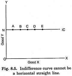
A little reflection will make it clear that an indifference curve on which those combinations of two goods lie that yield the same satisfaction to the consumer cannot take a shape other than downward-sloping to the right. If the indifference curve had the shape of a horizontal straight line (parallel to the X-axis), as in Fig. 8.5, that would mean as the amount of the good X was increased, while the amount of good Y remained the same, the consumer would remain indifferent as between various combinations. Y But this cannot be so if our assumption more of a commodity is better than less is to hold good.
According to assumption more of a commodity is better than less, the consumer always prefers a larger amount of a commodity to the smaller amount of it, other things being given. In Fig. 8.5 in various combinations such as A, B, C and D on indifference curve IC while the amount of good X is successively larger, the amount of good Y remains unchanged (= ON). If the consumer is to prefer a larger amount of good X to a smaller amount, then how he can be indifferent between combinations A, B, C, and D etc. It is thus concluded that indifference curve cannot be a horizontal straight line.
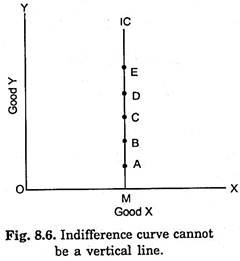
Likewise, indifference curve cannot be a vertical straight line, for a vertical straight line would mean that while the amount of good Y in the combination increases, the amount of good X remains the same. Thus, in Fig. 8.6, a vertical straight line IC is drawn on which are shown combinations A, B, C, D and E.
ADVERTISEMENTS:
While all these combinations contain the same amount of X, the amount of Y is successively larger. Thus, combinations A, B, C, D, etc. would not yield the same amount of satisfaction to the consumer and therefore cannot be the points of an indifference curve. We therefore conclude that indifference curve cannot be a vertical straight line too.
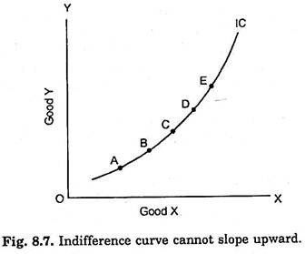
A third possibility for a curve is to slope upward to the right as in Fig. 8.7. But indifference curve cannot be of this shape too. Upward-sloping curve means that the amounts of both the goods increase as one moves to the right along the curve. If the indifference curve were upward sloping to the right, it would mean that combination which contains more of both the goods gave the same satisfaction to the consumer as the combination which had smaller amounts of both the goods. This is clearly invalid in view of our assumption more of a commodity is better than less. It follows therefore that indifference curve cannot slope upward to the right.
The last possibility for the curve is that it slopes downward to the right and this is the shape which the indifference curve can reasonable take. An indifference curve represents those combinations which give the same amount of satisfaction to the consumer and he is therefore indifferent between them.
In order that a consumer should get the same satisfaction from the various combinations of a curve and thus to maintain his indifference between them, then as the amount of good X is increased, the amount of good Y must be reduced. And this is what a downward-sloping curve indicates. A downward-sloping curve means that with every increase in the amount X, there is corresponding decrease in the amount of Y. As one moves to the right on such a curve, the various combinations on it will contain successively larger amount of X, but successively smaller amount of Y.
Thus, a consumer’s satisfaction can remain the same and he can be indifferent between the various combinations on a curve which slopes downward. We thus conclude that indifference curve slopes downward to the right. The slope of the indifference curve at its various points will depend upon how much of good Y the consumer is willing to give up for an additional unit of good X.
Property II. Indifference Curves are Convex to the Origin:
Another important property of indifference curves is that they are usually convex to the origin. In other words, the indifference curve is relatively flatter in its right-hand portion and relatively steeper in its left-hand portion. This property of indifference curves follows from assumption diminishing marginal rate of substitution, which is that the marginal rate of substitution of X for Y(MRSxy) diminishes as more and more of X is substituted for Y.
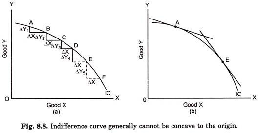
Only a convex indifference curve can mean a diminishing marginal rate of substitution of X for Y. If the indifference curve were concave to the origin it would imply that the marginal rate of substitution of X for Y increased as more and more of X was substituted for Y, as shown in Fig. 8.8 (a).
It will be clear from Fig. 8.8 (a) that as more and more of X is acquired, for each extra unit of X the consumer is willing to part with more and more of Y, that is, MRS, increases as more and more of X is substituted for Y. That, the concave indifference curve shows increasing MRSxy is also evident from Fig. 8.8 (b).
As we know that the slope at a point on an indifference curve shows the marginal rate of substitution of X for Y(MRS ) at that point, it will be seen that the slope at the point E on the indifference curve IC is greater than at point A (the tangent at E is steeper than the tangent at A). It therefore follows that MRSxy is greater at E than at A on the indifference curve IC. In other words, as more of X has been substituted for Y, MRSxy has increased.
The above Fig. 8.8 (a) and Fig. 8.8 (b) have been drawn to show that if indifference curves were concave to the origin, it would mean that the marginal rate of substitution of X for Y increased as the consumer obtained more and more of X in place of Y. But this clearly violates our fundamental assumption about the consumer’s behaviour which states that MRS declines as consumer substitutes more and more of X for Y. If the principle of diminishing marginal rate of substitution is valid, then the indifference curve cannot be concave to the origin.
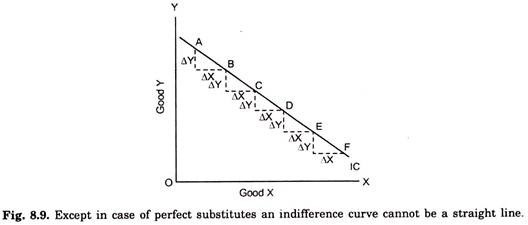
Likewise, indifference curve cannot be a straight-line, except when goods are perfect substitutes. A straight-line indifference curve would mean that MRSxy remains constant as more units of X are acquired in place of Y. As shown in Fig. 8.9 that on a straight-line indifference curve the amount of Y which the consumer is willing to give up for each additional unit of X remains the same as more and more of X is substituted for Y, that is, MRS remains constant.
Since MRS is equal to the slope of indifference curve at a point on it, and because a straight-line has the same slope throughout, therefore the straight line indifference curve will mean the same MRSxy, throughout. But, as said above, MRSxy, cannot remain constant except when goods happen to be perfect substitutes. Normal consumer’s behaviour reveals that when goods are less than perfect substitutes MRSxy, usually falls as more of good X is substituted for Y. It is therefore concluded that indifference curve cannot normally be a straight line.
The third possibility for indifference curve in this regard is that it may be convex to the origin and this is the shape which indifference curves normally possess. This is so because indifference curves being convex to the origin are consistent with the principle of diminishing marginal rate of substitution of X for Y. As shown in Fig. 8.4, when the indifference curve is convex to the origin, MRS, diminishes as more of X is substituted for Y. We therefore conclude that indifference curves are generally convex to the origin.
Our assumption regarding the diminishing MRSxy and the convexity of indifference curves is based upon the observation of actual behaviour of the normal consumer. When we come to discuss consumer’s equilibrium we shall see that indifference curves that are either concave or straight lines when viewed from the origin would suggest consumer’s behaviour which is contrary to that which is generally observed in real life.
If indifference curves were concave or straight lines, the consumer would succumb to monomania, that is, he would buy and consume only one good. We know that consumers in actual world do not generally buy and consume one good. It is for this reason that we reject indifference curves of concave or straight-line shapes and assume that indifference curves are normally convex to the origin.
The degree of convexity of an indifference curve depends upon the rate of fall in the marginal rate of substitution of X for Y. When two goods are perfect substitutes of each other, the indifference curve is a straight line on which marginal rate of substitution remains constant.
A straight-line indifference curve of perfect substitutes is shown in Fig. 8.9. The better substitutes the two goods are for each other, the closer the indifference curve approaches to the straight line so that when the two goods are perfect substitutes, the indifference curve is a straight line.
The greater the fall in marginal rate of substitution, the greater the convexity of the indifference curve. The less the ease with which two goods can be substituted for each other, the greater will be the fall in the marginal rate of substitution. In more usual cases, in which the two goods can be substituted for each other but are not perfect substitutes, the indifference curve will be convex to the origin. Perfect substitutes and perfect complements stand at opposite ends of the substitution scale. Between them are found most of the cases, for which indifference curves are convex to the origin.
Property III. Indifference Curves cannot Intersect Each Other:
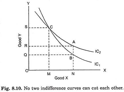
Third important property of indifference curves is that they cannot intersect each other. In other words, only one indifference curve will pass through a point in the indifference map. This property follows from assumptions more of a commodity is better than less and preference or indifference of a consumer are transitive. This property can be easily proved by first making the two indifference curves cut each other and then showing the absurdity or self- contradictory result it leads to.
In Fig. 8.10 two indifference curves are shown cutting each other at point C. Now take point A on indifference curve IC2 and point B on indifference curve IC1 vertically below A. Since indifference curve represents those combinations of two commodities which give equal satisfaction to the consumer, the combinations represented by points A and C will give equal satisfaction to the consumer because both lie on the same indifference curve IC2. Likewise, the combinations B and C will give equal satisfaction to the consumer; both being on the same indifference curve IC1.
If combination A is equal to combination C in terms of satisfaction, and combination B is equal to combination C, it follows that the combination A will be equivalent to B in terms of satisfaction. But a glance at Fig. 8.10 will show that this is absurd conclusion since combination A contains more of good Y than combination B, while the amount of good X is the same in both the combinations.
Thus, the consumer will definitely prefer A to B, that is, A will give more satisfaction to the consumer than B. But the two indifference curves cutting each other lead us to an absurd conclusion of A being equal to B in terms of satisfaction. We therefore conclude that indifference curves cannot cut each other.
Another point which is worth mentioning in this regard is that the indifference curves cannot even meet or touch each other or be tangent to each cut each other at a point. The meeting of two indifference curves at a point will also lead us to an absurd conclusion. The same argument holds good as developed above in the case of intersection.
Property IV. A Higher Indifference Curve Represents a Higher Level of Satisfaction than a Lower Indifference Curve:
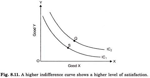
The last property of indifference curve is that a higher indifference curve will represent a higher level of satisfaction than a lower indifference curve. In other words, the combinations which ‘lie on a higher indifference curve will be preferred to the combinations which lie on a lower indifference curve.
Consider indifference curves IC1 and IC2 in Fig. 8.11. IC2 is a higher indifference curve than IC1 Combination Q has been taken on a higher indifference curve IC2 and combination S on a lower indifference curve IC1. Combination Q on the higher indifference curve IC2 will give a consumer more satisfaction than combinations S on the lower indifference curve IC1IC2 because the combination Q contains more of both goods X and Y than the combination S.
Hence by assumption more of a commodity is better than less, the consumer must prefer Q to S. And by transitivity assumption preference or indifferences of a consumer are transitive, he will prefer any other combination on IC2 (all of which are indifferent with Q) to any combination on IC, (all of which are indifferent with S). We, therefore, conclude that a higher indifference curve represents the higher level of satisfaction and combinations on it will be preferred to the combinations on a lower indifference curve.
Term Paper # 4. Indifference Curves of Perfect Substitutes and Perfect Complements:
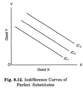
The degree of convexity of art indifference curve depends upon the rate of fall in the marginal rate of substitution of X for Y. As stated above, when two goods are perfect substitutes of each other, the indifference curve is a straight line on which marginal rate of substitution remains constant. Straight-line indifference curves of perfect substitutes are shown in Fig. 8.12.
The better substitutes the two goods are for each other, the closer the indifference curve approaches to the straight-line so that when the two goods are perfect substitutes, the indifference curve is a straight line. In case of perfect substitutes, the indifference curves are parallel straight lines because the consumer equally prefers the two goods and is welling to exchange one good for the other at a constant rate.
As one moves along a straight-line indifference curve of perfect substitutes marginal rate of substitution of one good for another remains constant. Examples of goods that are perfect substitutes are not difficult to find in the real world. For example, Dalda and Rath Vanaspati, two different brands of cold drink such as Pepsi Cola and Cola Cola. The greater the fall in marginal rate or substitution, the greater the convexity of the indifference curve.
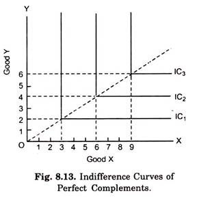
The less the ease with which two goods can be substituted for each other, the greater will be the fall in the marginal rate of substitution. At the extreme, when two goods cannot at all be substituted for each other, that is, when the two goods are perfect complementary goods, as for example gasoline and coolant in a car, the indifference curve will consist of two straight lines with a right angle bent which is convex to the origin as shown in Fig. 8.13 perfect complementary goods are used in a certain fixed ratio.
As will be seen in Fig. 8.13, the left-hand portion of an indifference curve of the perfect complementary goods is a vertical straight line which indicates that an infinite amount of Y is necessary to substitute one unit of X, and the right- hand portion of the indifference curve is a horizontal straight line which means that an infinite amount of X is necessary to substitute one unit of Y.
All this means that the two perfect complements are used in a certain fixed ratio and cannot be substituted for each other. In Fig. 8.13 two perfect complements are consumed in the ratio, 3X: 2Y. Complements are thus those goods which are used jointly in consumption so that their consumption increases or decreases simultaneously. Pen and ink, right shoe and left shoe, automobile and petrol, sauce and hamburger, typewriter and typists are some examples of perfect complements.
Term Paper # 5. Consumer’s Equilibrium: Maximising Satisfaction:
We are now in a position to explain with the help of indifference curves how a consumer reaches equilibrium position. A consumer is said to be in equilibrium when he is buying such a combination of goods as leaves him with no tendency to rearrange his purchases of goods. He is then in a position of balance in regard to the allocation of his money expenditure among various goods.
In the indifference curve technique the consumer’s equilibrium is discussed in respect of the purchases of two goods by the consumer. As in the cardinal utility analysis, in the indifference curve analysis also it is assumed that the consumer tries to maximize his satisfaction. In other words, the consumer is assumed to be rational in the sense that he aims at maximising his satisfaction.
Besides, we shall make the following assumptions to explain the equilibrium of the consumer:
(1) The consumer has a given indifference map exhibiting his scale of preferences for various combinations of two goods, X and Y.
(2) He has a fixed amount of money to spend on the two goods. He has to spend whole of his given money on the two goods.
(3) Prices of the goods are given and constant for him. He cannot influence the prices of the goods by buying more or less of them.
(4) Goods are homogeneous and divisible.
To show which combination of two goods, X and Y, the consumer will decide to buy and will be in equilibrium position, his indifference map and budget line are brought together. As seen above, while indifference map portrays consumer’s scale of preferences between various possible combinations of two goods, the budget line shows the various combinations which he can afford to buy with his given money income and given prices of the two goods.
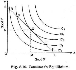
Consider Fig. 8.19 in which we depict consumer’s indifference map together with the budget line BL. Good X is measured on the X-axis and good Y is measured on the Y-axis. With given money to be spent and given prices of the two goods, the consumer can buy any combination of the goods which lies on the budget line BL. Every combination on the budget line BL costs him the same amount of money.
In order to maximise his satisfaction the consumer will try to reach the highest possible indifference curve which he could with a given expenditure of money and given prices of the two goods. Budget Constraint forces the consumer to remain on the given budget line, that is, to choose a combination from among only those which lie on the given budget line.
It will be seen from Fig. 8.19 that the various combinations of the two goods lying on the budget line BL and which therefore the consumer can afford to buy do not lie on the same indifference curve; they lie on different indifference curves. The consumer will choose that combination on the budget line BL which lies on the highest possible indifference curve. The highest indifference curve to which the consumer can reach is the indifference curve to which the budget line BL is tangent.
Any other possible combination of the two goods either would lie on a lower Good X indifference curve and thus yield less satisfaction or would be unattainable.
In Fig. 8.19 budget line BL is tangent to indifference curve IC3 at point Q. Since indifference curves are convex to the origin, all other points on the budget line BL, above or below the point Q, would lie on lower indifference curves. Take point R which also lies on the budget line BL and which the consumer can afford to buy. Combination of goods represented by R costs him the same as the combination Q.
But, as is evident, R lies on the lower indifference curve ICX and will therefore yield less satisfaction than Q. Likewise, point S also lies on the budget line BL but will be rejected in favour of Q since S lies on the indifference curve IC2 which is also lower than IC3 on which Q lies. Similarly, Q will be preferred to all the other points on the budget line RI, which lies to the right of Q on the budget line, such as T and H.
It is thus clear that of all possible combinations lying on budget line BL, combination Q lies on the highest possible indifference curve IC3 which yields maximum possible satisfaction. Of course, combinations king on indifference curves IC4 and IC5 will give greater satisfaction to the consumer than Q, but they are unattainable with the given money income and the given prices of the goods as represented by the budget line BL.
It is therefore concluded that with the given money expenditure and the given prices of the goods as shown by BL the consumer will obtain maximum possible satisfaction and will therefore be in equilibrium position at point Q at which the budget line BL is tangent to the indifference IC3. In this equilibrium position at Q the consumer will buy OM amount of good X and ON amount of good Y.
At the tangency point Q, the slopes of the budget line BL and indifference curve IC3 are equal. Slope of the indifference curve shows the marginal rate of substitution of X for Y (MRSxy), while the slope of the budget line indicates the ratio between the prices of two goods Px/Py. Thus, at the equilibrium point Q.
When the marginal rate of substitution of X for Y (MRSxy) is greater or less than the price ratio between the two goods, it is advantageous for the consumer to substitute one good for the other. Thus, at points R and S in Fig. 8.19, marginal rates of substitution (MRSxy) are greater than the given price ratio’, the consumer will substitute good X for good Y and will come down along the budget line BL. He will continue to do so until the marginal rate of substitution becomes equal to the price ratio, that is, the indifference curve becomes tangent to the given budget line BL.
On the contrary, marginal rates of substitution at points H and T in Fig. 8.19 are less than the given price ratio. Therefore, it will he to the advantage of the consumer to substitute good Y for good X and accordingly move up the budget line BL until the MRS rises so as to become equal to the given price ratio.
We can therefore express the condition for the equilibrium of the consumer by either saying that the given budget line must be tangent to the indifference curve, or the marginal rate of substitution of good X for good Y must be equal to the ratio between the prices of the two goods.
Second Order Condition for Consumer Equilibrium:
The tangency between the given budget line and an indifference curve or, in other words, the equality between MRSxy, and the price ratio is a necessary but not a sufficient condition of consumer’s equilibrium. The second order condition must also be fulfilled. The second order condition is that at the point of equilibrium indifference curve must be convex to the origin, or to put it in another way, the marginal rate of substitution of X for Y must be falling at the point of equilibrium.
It will be noticed from Fig. 8.19 above that the indifference curve IC3 is convex to the origin at Q. Thus at point Q both conditions IC3 of equilibrium are satisfied. Point Q in Fig. 8.19 is the optimum or best choice for the consumer and he will therefore be in stable equilibrium at Q.
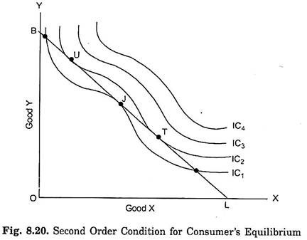
But it may happen that while budget line is tangent to an indifference curve at a point but the indifference curve may be concave at that point. Take for instance, Fig. 8.20 where indifference curve IC1 is concave to the origin around the point J. Budget line BL is tangent to the indifference curve IC, at point J and MRSxy, is equal to the price ratio, Px/Py.
But J cannot be a position of equilibrium because satisfaction would not be maximise here. Indifference curve IC1 being concave at the tangency point J, there may be some points on the given budget line BL such as U and T, which will be on indifference curve higher than IC1. Thus, consumer by moving along the given budget line BL can go to points such as 11 and T, and obtain greater satisfaction than at J.
We therefore conclude that for the consumer to be in the following two conditions are required:
1. A given budget line must be tangent to indifference curve, or marginal rate of substitution of X for Y (MRSxy) to the price ratio of the two goods Px/Py.
2. Indifference curve must be convex to the origin at the point of tangency.
The above explanation of consumer’s equilibrium in regard to the allocation of his money expenditure on the purchases of two goods has been made entirely in terms of relative preferences of the various combinations of two goods. In this indifference curve analysis of consumer’s equilibrium no use of marginal utility concept has been made which implies that satisfaction or utility obtained from the goods is measurable in the cardinal sense.
Term Paper # 6. Three Demand Theorems Based on Indifference Curve Analysis:
It follows from above that, indifference curve analysis enables us to enunciate a more general law of demand in the following composite form, consisting of three demand theorems to which the Marshallian law of demand constitutes a special case:
(а) The quantity demanded of a good varies inversely with price when the income effect is positive or nil.
(b) The quantity demanded of a good varies inversely with price when the income effect for the good is negative but is weaker than the substitution effect.
(c) The quantity demanded of a good varies directly with price when the income effect for the good is negative and this negative income effect of a change in price is larger than the substitution effect.
In the first or second case, the Marshallian law of demand holds good and we get a downward sloping demand curve. When the third case occurs, we get a Giffen good of positively sloping demand curve. Marshallian law of demand does not hold true in the third case. Marshall mentioned Giffen-good case as an exception to his law of demand.
Thus the indifference curve analysis is superior to Marshallian analysis in that it yields a more general law of demand which covers the Giffen-good case. The explanation for the occurrence of a Giffen good is that in its case the negative income effect outweighs the substitution effect. Since Marshall ignored the income effect of the change in price, he could not provide a satisfactory explanation for the reaction of the consumer to a change in the price of a Giffen good.
However, it may be pointed out that it is very hard to satisfy the above mentioned third conditions for the occurrence of the Giffen good, namely, the consumer must be spending a very large proportion of his income on an inferior good. Therefore, although Giffen case is theoretically possible the chance of its occurrence in the actual world is almost negligible.
This is because consumption of the people is generally diversified so that people spend a small proportion of their income on a single commodity with the result that price-induced income effect even when negative is generally small and cannot therefore outweigh the substitution effect.
Marshall believed that quantity demanded in actual practice could vary directly with price, and Sir Robert Giffen is said to have actually observed this phenomenon. But there is a controversy about the interpretation of this so-called Giffen phenomenon. But from our analysis, it is clear that, Giffen good case can occur in theory.
When negative income effect of the fall in the price of an inferior good is larger than substitution effect we get a positively-sloping demand curve of Giffen good. Thus Giffen good is theoretically quite possible. But, since income effect of the change in price of a single commodity in the real world is small, the negative income effect of the change in price of an inferior good is too weak to swamp the substitution effect and therefore Giffen case, although theoretically conceivable, rarely occurs in practice.
Term Paper # 7. Derivation of Individual’s Demand Curve from Indifference Curve Analysis:
Price consumption curve traces the effect of a change in price on the quantity demanded of a good. But price consumption curve does not directly relate price with quantity demanded. In indifference curve diagram price is not explicitly shown on the Y-axis. On the other hand, demand curve directly relates price with quantity demanded, price being shown on Y-axis and quantity demanded on the X-axis.
A demand curve shows how much quantity of a good will be purchased or demanded at various prices, assuming that tastes and preferences of a consumer, his income, prices of all related goods remain constant. This demand curve showing explicit relationship between price and quantity demanded can be derived from price consumption curve of indifference curve analysis.
In Marshallian utility analysis, demand curve was derived on the assumptions that utility was quantitatively measurable and marginal utility of money remained constant with the change in price of the good. In the indifference curve analysis, demand curve is derived without making these dubious assumptions.
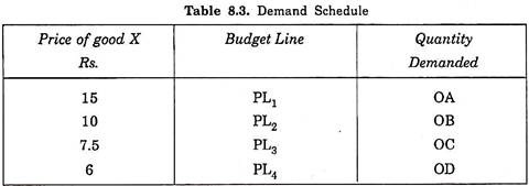
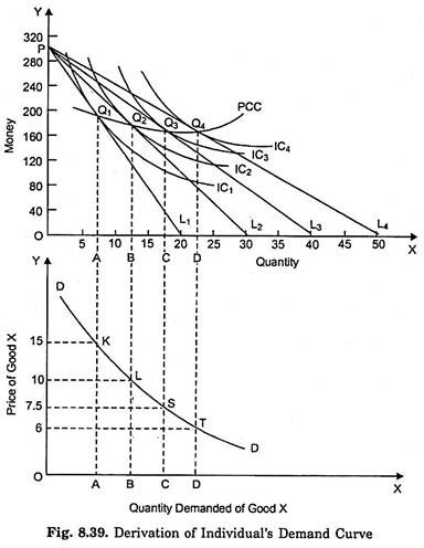
Let us suppose that a consumer has got income of Rs. 300 to spend on goods. In Fig. 8.38 money is measured on the Y-axis, while the quantities of the good X whose demand curve is to be derived is measured on the X-axis. An indifference map of a consumer is drawn along with the various budget lines showing different prices of the good X. Budget line PL, shows that price of the good X is Rs. 15 per unit.
As the price of good X falls from Rs. 15 to Rs. 10, the budget line shifts to PL2. Budget line PL2 shows that price of good X is Rs. 10. With a further fall in price to Rs. 7.5 the budget line takes the position PL3. Thus PL3 shows that price of good X is Rs. 7.5. When the price of good X falls to Rs. 6, PL4 is the relevant budget line.
The various budget lines obtained are shown in the column 2 of the following table. Tangency points between the various budget lines and indifference curves, which when joined together by a line constitute the price consumption curve which shows the amounts of good X purchased or demanded at the corresponding prices.
With the budget line PL1 the consumer is in equilibrium at point Q, on the price consumption curve at which the budget line PL, is tangent to indifference curve IC1. In his equilibrium position at Q, the consumer is buying OA units of the good X. In other words, it means that the consumer demands OA units of good X at price Rs. 15.
When price falls to Rs. 10 and thereby the budget line shifts to PL2, the consumer comes to be in equilibrium at point Q2 of the price-consumption curve where the budget line PL2 is tangent to indifference curve IC2. At Q2, the consumer is buying OB units of good X. In other words, the consumer demands OB units of the good X at price Rs. 10.
Likewise, with budget lines PL3 and PL4, the consumer is in equilibrium at points Q3 and Q4 of price consumption curve and is demanding OC units and OD units of good X at price Rs. 7.5 and Rs. 6 respectively. It is thus clear that from the price consumption curve we can get information which is required to draw the demand curve showing directly the amounts demanded of the good X against various prices.
With the above information we draw up the demand schedule in the table given as follows:
The adjoining demand schedule which has been derived from the indifference curves diagram can be easily converted into a demand curve with price shown on the Y-axis and quantity demanded on the X-axis. It will be easier if this demand curve is drawn rightly below the indifference curves diagram. This has been done so in Fig. 8.39. In the diagram at the bottom, on the X-axis the quantity demanded is shown as in indifference curves diagram above, but on the Y-axis in the diagram at the bottom price per unit of the good X is shown instead of total money.
In order to obtain the demand curve, various points K, L, S and T representing the demand schedule of the above table are plotted. By joining the points K, L, S and T we get the required demand curve DD.
Term Paper # 8. Superiority of Indifference Curve Analysis:
We are now in a position to compare the indifference curve analysis with Marshallian cardinal utility analysis. It is now widely believed that indifference curve analysis makes a define improvement upon the Marshallian cardinal utility analysis. It has been asserted the whereas Marshallian cardinal utility analysis assumes ‘too much’ it explains ‘too little’. On the other hand, the’ indifference curve analysis explains more by taking fewer as well as less restrictive assumptions.
It may be noted that there are some similarities in these two theories of demand:
1. First, both these theories assume that consumers are rational and therefore try to maximize utility or satisfaction.
2. Second, both these theories use psychological or introspective method to explain consumer’s behaviour.
3. Thirdly, both these theories of demand assume in some form diminishing marginal utility or desire for a commodity as a consumer takes more units of a commodity. In this connection it is generally believed that the principle of diminishing marginal rate of substitution is similar to the law of diminishing marginal utility of Marshallian utility analysis.
After having pointed out the similarities between the two types of analysis, we now turn to study the differences between the two and to show how far indifference curve analysis is superior to the Marshallian cardinal utility analysis.
Dissimilarities in these two theories of demand:
1. Ordinal vs. Cardinal Measurability of Utility:
In the first place, Marshall assumes utility to be cardinally measurable. In other words, he believes that utility is quantifiable, both in principle and in actual practice. According to this, the consumer is able to assign specific amounts to the utility obtained by him from the consumption of a certain amount of a good or a combination of goods. Further, these amounts of utility can be added and compared in the same manner as weights, lengths, heights, etc.
According to the critics, the assumption of cardinal measurement of utility is very strong, it demands too much from the human mind. They assert that utility is a psychological feeling and the cardinal measurement of utility assumed by Marshall and others is therefore unrealistic. Critics hold that the utility possesses only ordinal magnitude and cannot be expressed in cardinal terms.
Therefore, the indifference curve analysis assumes that utility is merely orderable and not quantitative. In other words, indifference curve technique assumes what is called ‘ordinal measurement of utility’. According to this, the consumer is capable of comparing different utilities or satisfactions in the sense whether one level of satisfaction is equal to, lower than, or higher than another.
The advocates of indifference curve technique assert that for the purpose of explaining consumer’s behaviour and deriving the law of demand, it is quite sufficient to assume that the consumer is able to rank his preferences consistently. It is obvious that the ordinal measurement of utility makes a less strong assumption and sounds more realistic than cardinal measurement of utility. This shows that the indifference curve analysis of demand which is based upon the ordinal utility hypothesis is superior to Marshall’s cardinal utility analysis.
2. Analysis of Demand without Assuming Constant Marginal Utility of Money:
Another distinct improvement made by indifference curve technique is that unlike Marshall it explains consumer’s behaviour and derives demand theorem without the assumption of constant marginal utility of money. In indifference curve analysis, it is not necessary to assume constant marginal utility of money.
It has already been seen; Marshall assumed that the marginal utility of money remained constant when there occurred a change in the price of a good. The Marshallian demand analysis based upon constancy of marginal utility of money is not applicable to multi-commodity model.
In words, the Marshallian demand theorem cannot genuinely be derived from the marginal utility hypothesis except in one commodity model, without contradicting the assumption of constant marginal utility of money. On the other hand, indifference curve technique using ordinal utility hypothesis can validly derive the demand theorem without the assumption of constant marginal utility of money. In fact, giving up the assumption of constant marginal utility of money enables the indifference curve analysis to enunciate a more general demand theorem.
3. Greater Insight into Price Effect:
The superiority of indifference curve analysis further lies in the fact that it makes greater insight into the effect of the price change on the demand for a good by distinguishing between income and substitution effects. The indifference curve technique splits up the price effect analytically into its two component parts- substitution effect and income effect.
The distinction between the income effect and the substitution effect of a price change enables us to gain a better understanding of the effect of a price change on the demand for a good. The amount demanded of a good generally rises as a result of the fall in its price due to two reasons. First, because real income rises as a result of the fall in price (income effect) and, secondly, because the good whose price falls becomes relatively cheaper than others and therefore the consumer substitutes it for others (substitution effect).
But, Marshall by assuming constant marginal utility of money ignored the income effect of a price change. He failed to understand the composite character of the effect of a price change. Thus JR. Hicks writes, “The distinction between direct and indirect effects of a price change is accordingly left by the cardinal theory as an empty box, which is crying out to be filled. But it can be filled”.
Further, Tapas Majumdar writes “The efficiency and precision with which Hicks-Allen approach can distinguish between the ‘income’ and ‘substitution’ effects of a price change really leaves the cardinalist argument in a very poor state indeed.”
4. Deriving a more General and Adequate ‘Demand Theorem’:
A distinct advantage of the technique of dividing the effect of a price change into income and the substitution effects employed by the indifference curve analysis is that it enables us to enunciate a more general and a more inclusive theorem of demand than the Marshallian law of demand. In the case of most of the normal goods in the world, both the income effect and the substitution effect work in the same direction, that is to say, they tend to increase the amount demanded when the price of a good falls.
The income effect ensures that when the price of a good falls, the consumer buys more of it because he can now afford to buy more of it; the substitution effect ensures that he buys more of it because it has now become relatively cheaper and is, therefore, profitable to substitute it for others. This thus accounts for the inverse price- demand relationship (Marshallian law of demand) in the case of normal goods.
When a certain good is regarded by the consumer to be an inferior good, he will tend to reduce its consumption as a result of the increase in his income. Therefore, when the price of an inferior good falls, the income effect so produced would work in the opposite direction to that of the substitution effect.
But so long as the inferior good in question does not claim a very large proportion of consumer’s total income, the income effect will not be strong enough to outweigh the substitution effect. In such a case therefore the net effect of the fall in price will be to raise the amount demanded of the good. It follows that even for most of the inferior goods, the Marshallian law of demand holds good as in case of normal goods.
But it is possible that there may be inferior goods for which the income effect of a change in price is larger in magnitude than the substitution effect. This is the case of Giffen goods for which the Marshallian law of demand does not hold good. In such cases the negative income effect outweighs the substitution effect so that the net effect of the fall in price of the good is the reduction in demand for it. Thus, amount demanded of a Giffen good varies directly with price.
It is clear from above that by breaking the price effect into income effect and substitution effect, the indifference curve analysis enables us to arrive at a general and a more inclusive theorem of demand in the following composite form:
(a) The demand for a commodity varies inversely with price when the income effect for that commodity is nil or positive as substitution effect is always present and tends to increase the quantity demanded of the commodity whose price falls and vice-versa.
(b) The demand for a commodity varies inversely with price when the income effect is negative but this negative income effect of the price change is smaller than the substitution effect.
(c) The demand for a commodity varies directly with price when the income effect is negative and this negative income effect of the price change is larger than the substitution effect.
In the case of (a) and (b) the Marshallian law of demand holds while in case of (c) we have a Giffen good case which is exception to the Marshallian law of demand. Marshall could not account for ‘Giffen Paradox’. Marshall was not able to provide explanation for ‘Giffen Paradox’ because by assuming constant marginal utility of money, he ignored the income effect of the price change.
5. Indifference Curve Analysis can Explain Substitute and Complementary Relationships between Goods:
Marshall’s cardinal utility analysis is based upon the hypothesis of independent utilities. This means that the utility which the consumer derives from any commodity is a function of the quantity of that commodity and of that commodity alone. In other words, utility obtained by the consumer from a commodity is independent of that derived from any other. By assuming independent utilities Marshall completely bypassed the relation of substitution and complementarily between commodities.
Demand analysis based upon the hypothesis of independent utilities leads us to the conclusion “that in all cases a reduction in the price of one commodity only will either result in an expansion in the demand for all other commodities or in a contraction in the demands for all other commodities”. But his is, quite contrary to the common cases found in the real world.
In the real world, it is found that as a result of the fall in price of a commodity the demand for some commodities expands while the demand for others contracts. We thus see that Marshall’s analysis based upon ‘independent utilities’ does not take into account the complementary and substitution relations between goods. This is a great flaw in Marshall’s cardinal utility analysis.
On the other hand, this flaw is not present in Hicks-Allen indifference curve analysis which does not assume independent utilities and duly recognizes the relation of substitution and complementarily between goods. Hicks-Allen indifference curve technique by recognizing interdependence of utilities is in a better position to explain related goods. By breaking up price effect into substitution and income effects by employing the technique of compensating variation income, Hicks succeeded in explaining complementary and substitute goods in terms of substitution effect alone.
6. Analysing Consumer’s Demand with Less Restrictive and Fewer Assumptions:
It has been shown above that both the Hicks-Allen indifference curve theory and Marshall’s cardinal theory arrive at the same condition for consumer’s equilibrium. Hicks-Allen condition for consumer’s equilibrium, that is, MRS must be equal to the price ratio amounts to the same thing as Marshall’s proportionality rule of consumer’s equilibrium. But even here indifference curve ordinal approach is an improvement upon the Marshall’s cardinal theory in so far as the former arrives at the same equilibrium condition with less restrictive and fewer assumptions.
Dubious Assumptions such as:
(i) Utility is quantitatively measurable,
(ii) Marginal utility of money remains constant, and
(iii) Utilities of different goods are independent of each other, on which Marshall’s cardinal theory is based, are not made in indifference- curve’s ordinal utility theory.
Term Paper # 9. Is Indifference Curve Analysis “The Old Wine in a New Bottle”?
But superiority of indifference curve theory has been denied by some economists; foremost among them are Prof. D.H. Robertson, F.H. Knight, and W.E. Armstrong. Prof. Knight Remarks, “indifference curve analysis of demand is not a step forward; it is in fact a step backward.” Prof. D.H. Robertson is of the view that the indifference curve technique is merely “the old wine in a new bottle”.
The indifference curve analysis, according to him, has simply substituted new concepts and equations in place of the old ones, while the essential approach of the two types of analyses is the same. Instead of the concept of ‘utility’, the indifference curve technique has introduced the term ‘preference’ and scale of preferences.
In place of cardinal number system of one, two, three, etc., which is supposed to measure the amount of utility derived by the consumer, the indifference curves have the ordinal number system of first, second, third, etc., to indicate the order of consumer’s preferences. The concept of marginal utility has been sub-situated by the concept of marginal rate of substitution. And against the Marshallian ‘proportionality rule’ as a condition for consumer’s equilibrium, indifference curve approach has advanced the condition of equality between the marginal rate of substitution and the price ratio.
Expressing the view that, the concept of marginal rate of substitution in indifference curve analysis, represents the reintroduction of the concept of marginal utility in demand analysis.
Prof. Robertson says: “In his earlier book Value and Capital Hick’s treatment involved making an assumption about the convexity of those ‘indifference curves’ which appeared to some of us to involve reintroduction of marginal utility in disguise.”
Thus, according to Prof. Robertson the use of marginal rate of substitution implies the presence of cardinal element in indifference curve technique. In going from one combination to another on an indifference curve, the consumer is assumed to be able to tell what constitutes his compensation in terms of a good for the loss of a marginal unit of’ another good, that is, he is able to tell his marginal rate of substitution of one good for another.
Thus, it has, therefore, been held that the concept of marginal rate of substitution and the idea of indifference based upon it essentially involves an admission that utility is quantifiable in principle. However, this is not correct interpretation of the concept of marginal rate of substitution. As Hicks has pointed out, we need not assume measurability of marginal utilities in principle in order to know the marginal rate of substitution.
He says, “All that we shall be able to measure is what the ordinal theory grants to be measurable-namely the ratio of the marginal utility of one commodity to the marginal utility of another.”
This means that MRS can be obtained without actually measuring marginal utilities. If a consumer, when asked, is prepared to accept 4 units of good Y for the loss of one marginal unit of X, MRS of X for Y is 4: 1. ‘We can thus directly derive the ratio indicating MRS without measuring marginal utilities by offering him how much compensation in terms of good Y the consumer would accept for the loss of a marginal unit of X.
It has been further contended by Robertson and Armstrong that it is not possible to arrive at the Hicksian principle of diminishing marginal rate of substitution without making use of the ‘Marshallian framework’ of the concept of marginal utility and the principle of diminishing marginal utility. It is asked why MRS of X for Y diminishes as more and more of X is substituted for Y?
The critics point out that the marginal rate of substitution (MRS) diminishes and the indifference curve becomes convex to the origin, because as the consumer’s stock of X increases, the marginal utility of X falls and that of Y increases. They thus hold that Hicks and Allen have not been able to derive the basic principle of diminishing marginal rate of substitution independently of the law of diminishing marginal utility.
They contend that by a stroke of terminological manipulation, the concept of marginal utility has been relegated to the background, but it is there all the same. They, therefore, assert that “the principle of diminishing marginal rate of substitution is as much determinate or indeterminate as the poor law of diminishing marginal utility”.
However, even this criticism of indifference curve approach advanced by the defenders of the Marshallian cardinal utility analysis is not valid. The derivation of marginal rate of substitution does not depend upon the actual measurement of marginal utilities.
While the law of diminishing marginal utility is based upon the cardinal utility hypothesis (i.e., utility is quantifiable and actually measurable), the principle of marginal rate of substitution is based upon the ordinal utility hypothesis (i.e., utility is mere orderable). As a consumer gets more and more units of good X, his strength of desire for it (though we cannot measure it in itself) will decline and therefore he will be prepared to forgo less and less of Y for the gain of a marginal unit of X.
It is thus clear that the principle of diminishing marginal rate of substitution is based upon purely ordinal hypothesis and is derived independently of cardinal concept of marginal utility, though both laws reveal essentially the same phenomenon. The derivation of the principle of diminishing marginal rate of substitution by using ordinal utility hypothesis and being quite independent of the concept of marginal utility is a great achievement of the indifference curve analysis.
We therefore agree with Prof. Hicks who claims that “the replacement of the principle of diminishing marginal utility by the principle of diminishing marginal rate of substitution is not a mere translation. It is a positive change in the theory of consumer’s demand”.
It follows from what has been said above that indifference curve analysis of demand is an improvement upon the Marshallian utility analysis and the objections that the former too involves cardinal elements are groundless. It is of course true that the indifference curve analysis suffers from some drawbacks and has been criticized on various grounds, as explained below, but as far as the question of indifference curve technique versus Marshallian utility analysis is concerned, the former is decidedly better.
Term Paper # 10. Critique of Indifference Curve Analysis:
Indifference curve analysis has come in for criticism on several grounds. In the first place, it is argued that the indifference curve approach for avoiding the difficulty of measuring utility quantitatively is forced to make unrealistic assumption that the consumer possesses complete knowledge of his whole scale of preferences or indifference map. The indifference curve approach, so to say, falls from the frying pan into the fire.
The indifference curve analysis envisages a consumer who carries in his head innumerable possible combinations of goods and relative preferences in respect of them. It is argued: Is not this carrying into his head all his scales of preferences too formidable a task for a real human being? Hicks himself admits this drawback.
When revising his demand theory based on indifference curves, he says that “one of the most awkward of the assumptions into which the older theory appeared to be impelled by its geometrical analogy was the notion that the consumer is capable of ordering all conceivable alternatives that might possibly be presented to him all the positions which might be represented by points on his indifference map. This assumption is so unrealistic that it was bound to be a stumbling block.” This is one of the reasons why Hicks has given up indifference curves in his Revision of Demand Theory.
Further, another unrealistic element is present in indifference curve analysis. It is pointed out that such curves include even the most ridiculous combinations which may be far removed from his habitual combinations. For example, while it may be perfectly sensible to compare whether three pairs of shoes and six shirts would give a consumer as much satisfaction as two pairs of shoes and seven shirts, the consumer will be at a loss to know and compare the desirability of an absurd combination such as eight pairs of shoes and one shirt.
The way the indifference curves are constructed, they include absurd combinations like the one just indicated. A further shortcoming of the indifference curve technique is that it can demonstrate and analyses consumer’s behaviour effectively only in simple cases, especially those in which the choice is between the quantities of two goods only. In order to demonstrate the case of three goods, three-dimensional diagrams are needed which are difficult to understand and handle.
When more than three goods are involved, geometry altogether fails and recourse has to be made to the complicated mathematics which often tends to conceal the economic aspect of what is being done. Prof. Hicks also admits this shortcoming of indifference curve technique.
Another demerit of the geometrical nature of indifference curve analysis is that it involves the assumption of continuity “a property which the geometrical field does have, but which the economic world in general does not”. The real economic world exhibits discontinuity and it is quite unrealistic and analytically bad if we do not recognize it. This is why Hicks too has given up the assumption of continuity in his later work ‘A Revision of Demand Theory.
Another important criticism against Hicks-Allen ordinal theory of demand is that it cannot formalise consumer’s behaviour when uncertainty or risk is present. In other words, consumer’s behaviour cannot be explained by ordinal utility theory when he has to choose among alternatives involving risk or ‘uncertainty of expectation’. Von Neumann and Morgenstern and also Armstrong have asserted that “while cardinal utility theory can, the ordinal utility theory cannot formalise consumer’s behaviour when we introduce “uncertainty” of expectations with regard to the consequences of choice.”
Further, Prof. Samuelson has criticized the indifference curve approach for being predominantly introspective. Prof. Samuelson himself has developed a behaviorist method of deriving the theory of demand. He seeks to enunciate demand theorem from observed consumer’s behaviour. He regards the behavioristic approach, as being ‘scientific’. His theory is based upon the strong-ordering hypothesis, namely, ‘choice reveals preference.’ Samuelson thinks that his theory removes the last vestiges of the psychological analysis in the explanation of consumer’s demand.
