
In this article we will discuss about the theory of optimum tariff.
It is, of course, true that tariff, and in certain situations may fail to improve the terms of trade of a given country. There is, however, a widespread belief that tariffs can improve the terms of trade. This leads to a vital question, viz., to what extent a country can go on increasing tariffs, improve its terms of trade and maximise the economic welfare.
Tariffs result in gain for the tariff-imposing home country in the form of improvement in the terms of trade. At the same time, tariffs involve cost in the form of reduction in the volume of exports and imports. So long as the gain from tariffs is more than the cost of it, the welfare of the tariffs-imposing country increases and it is worthwhile for it to raise tariff.
In case the cost of tariffs for the society is more than the gain from tariffs, there may be reduction in the level of economic welfare and the worsening of the terms of trade.
ADVERTISEMENTS:
In such a situation, it is appropriate for the tariff-imposing country to reduce tariff. The point of optimum tariff is reached when tariff does not further increase the net benefit to the given country and a level of economic welfare has become maximum. In the words of Sodersten, “…. the tariff that maximises a country’s welfare is called the optimum tariff.”
The point of optimum tariffs is determined where the trade indifference curve of the tariff-imposing home country becomes tangent to the offer curve of the foreign country. This can be shown through Fig. 15.9.
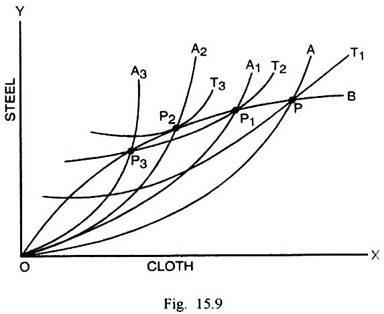
In Fig. 15.9 originally OA is the offer curve of home country A and OB is the offer curve of foreign country B. T1, T2 and T3 are the trade indifference curves of country A. Before the imposition of tariff, the exchange takes place at P. This point lies on the trade indifference curve T1. As tariff is imposed, the offer curve of county A shifts to OA1 and exchange takes place at P1. This point occurs at the higher trade indifference curve T2.
ADVERTISEMENTS:
Thus tariff results in an improvement in terms of trade, on the one hand, and increases the level of welfare on the other. If there is a further increase in tariff, country A’s offer curve shifts to OA2 and given the offer curve OB of country B, the exchange takes place at P2. This point occurs at the higher trade indifference curve T3. P2 is the point of tangency between the trade indifference curve T3 and foreign country B’s offer curve OB. Compared with point P1, there is a further improvement in the terms of trade and increase also in the level of welfare.
In case, country A raises the tariff still further, its offer curve shifts to the left to OA3. Given the offer curve of country B as OB, exchange takes place now at P3. This point shows that terms of trade improve further but this point lies on a lower trade indifference curve T2.
Although the terms of trade in this situation improve, yet there is worsening in respect of the level of welfare. In such a situation, it is appropriate for the home country to reduce tariff and move back to the point P2 where the welfare is maximum. Thus P2 is the point of optimum tariff which corresponds with the maximisation of welfare.
Optimum Tariff with Retaliation:
ADVERTISEMENTS:
In the above analysis, the home country continues to raise tariffs and improve its terms of trade. It has been implicitly assumed that foreign country does not retaliate. In actual reality, the possibility of retaliation cannot be ruled out. The impact of imposition of tariffs by the two trading countries upon their terms of trade and the level of welfare can be shown through Fig. 15.10.

In Fig. 15.10, OA and OB are the free trade offer curves of countries A and B respectively. P is the point of exchange and the terms of trade for the home country A are measured by the slope of line OP. This point lies on the trade indifference curves T1 and T1’ of countries A and B respectively. So point P also indicates the respective welfare levels in these countries in the pre-tariff situation.
If country A imposes tariff so that its offer curve shifts to OA1 while country B does not enforce any retaliatory tariff, P1 is the point of optimum tariff for A. At this point of exchange, the higher trade indifference curve T2 of country A is tangent to the offer curve OB of country B. There is an improvement in terms of trade as well as an increase in welfare of the tariff-imposing home country.
If country B had imposed tariff first without provoking country A to retaliation, the point of exchange would have shifted from P to P2. This would have been the point of optimum tariff for B because of tangency between its higher trade indifference curve T2 and the offer curve OA of country A. The point P2 shows an improvement in terms of trade and increase in the level of welfare for B.
In case the tariff action of A is followed by the retaliatory tariff action of country B, their respective offer curves OA1 and OB1 intersect each other at P3. The terms of trade for both the countries are exactly the same as at the pre-tariff position P. The point P3 is the optimum tariff situation because the trade indifference curves T3 and T3‘ are tangent to the offer curve of each other at this point.
However, the point P3 lies on the lower trade indifference curves of the two countries, compared with the tariff situations (P1 and P2) in the absence of retaliation. So tariff has left their terms of trade unchanged but has worsened the level of welfare in both the countries. The above analysis shows that both the countries in the ultimate analysis are likely to lose due to tariff. Johnson has, however, not supported such a general conclusion.
In his words, “…whatever the final equilibrium point, one country must lose under tariff as compared with free trade, since gain depends on obtaining an improvement in the terms of trade sufficient to outweigh the loss of trade volume, and this is impossible for both countries simultaneously, and both countries may lose…….. but it is not necessarily true that both will lose.”
The tariff action, particularly retaliatory tariff may or may not permit the improvement in terms of trade, but one thing is definite that it will reduce sharply the volume of trade and lower the level of welfare. In view of this, it is better for both the trading countries to avoid disastrous, beggar-my- neighbour tariff policies.
ADVERTISEMENTS:
The lowering down of tariff walls can, no doubt, affect adversely the terms of trade but the expansion in trade volume and consequent increase in welfare will certainly be highly desirable from the point of view of both the trading countries.
The Optimum Tariff Formula:
The economists and financial administrators have remained concerned with determining the rate of tariff that can ensure the improvement in terms of trade consistent with the maximization of welfare. They have preferred to call such a rate of tariff as the optimum rate of tariff. The economists, including Robert Heller, Scammel and Kindelberger have attempted to work out a precise formula for specifying the optimum rate of tariff.
Kindelberger has stated the formula for optimum tariff in the following form:
ADVERTISEMENTS:
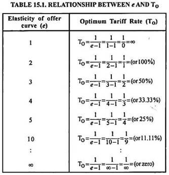
TO = 1/ (e-1)
Here TO denotes the optimum rate of tariff and e stands for the elasticity of the offer curve of the foreign country at the specific point.
The co-efficient e or the elasticity of offer curve can be measured as below:
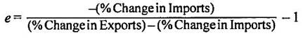
ADVERTISEMENTS:
The rate of optimum tariff can be derived geometrically with the help of Fig. 15.11.
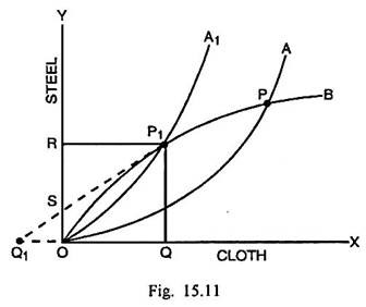
In Fig. 15.11, OA is the offer curve of tariff-imposing home country A and OB is the offer curve of the foreign country B. P is the original point of exchange and P1 is the point of exchange subsequent to the imposition of tariff. It is assumed that P1 is the point of optimum tariff.
The slope of the offer curve at point P1 is measured by the tangent drawn to OB at P1. It meets the horizontal scale produced in the backward direction at Q1. The optimum tariff at P1 is (OQ1/ OQ). As OQ = RP, therefore, the optimum tariff can be expressed as OQ1/RP1. Since the Δs SQ1O and SP1R are similar, OQ1/ RP1 equals OS/SR.
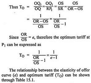
ADVERTISEMENTS:
From the Table 15.1 it follows that the optimum tariff rate that can maximise welfare goes on diminishing as the co-efficient e increases and vice- versa. It implies that there is an inverse relation between the elasticity of the offer curve of country B and the optimum tariff rate for country A. In the extreme situation, when the elasticity of the offer curve of foreign country is infinite the tariff-imposing home country will fail to bring about an improvement in its terms of trade. This can be shown through Fig. 15.12.
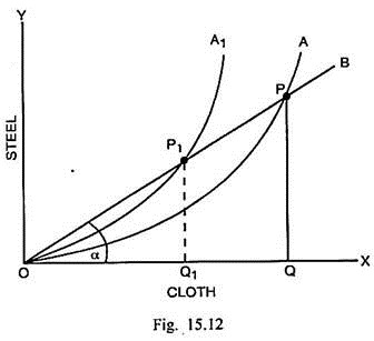
In Fig. 15.12, OA is originally the offer curve of country A and OB is perfectly elastic (e = α) offer curve of country B. The exchange takes place at P and country A imports PQ quantity of steel in exchange of the export of OQ quantity of cloth.
The TOT at P for country A = (QM/QX) = (PQ/OQ) = Slope of Line OP = Tan α. As country A imposes tariff, its offer curve shifts to OA1. In this case, exchange takes place at P1 where P1Q1 quantity of steel is imported against the export of OQ1 quantity of cloth. The TOT for country A at P1 = (QM/QX) = (PQ1/OQ1) = Slope of Line OP1 = Tan α1.
Slope of Line OP1 = Tan α. Since TOT at P and P1 are both measured by constant Tan α, the home country cannot improve the terms of trade through tariff. There is only reduction in the volume of trade and consequent decline in the level of welfare.
If the above exceptional case is left out, the offer curve of foreign country can assume the elasticity less than unity, equal to unity and more than unity. The implications of such magnitudes of e upon the terms of trade and welfare (or optimum tariff on the whole) can be discussed through Fig. 15.13.
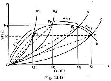
In Fig. 15.13 OA is originally the offer curve of home country. OB, on the other hand, is the offer curve of foreign country B. The entire span of this curve consists of three elasticity ranges. In the OP2 range, the elasticity is greater than unity (e > 1). In the P2P1 range, the elasticity is equal to unity (e = 1). In the PP1 range, the elasticity is less than unity (e < 1).
As country A goes on raising tariff, the offer curve of home country continues to shift to the left from OA and OA1, OA2 and OA3. The point of exchange shifts from P to P1, P2 and P3 respectively and there is improvement in the terms of trade for the home country. The point of exchange P3 is preferable to P because country A can import OR quantity of steel as much as in the pre-tariff exchange position P by exporting only OQ3 quantity of cloth.
At P, country A was required to export OQ quantity of cloth for importing OP quantity of steel. But compared to P3, the trade equilibrium point P2 is preferable. Although the terms of trade at P2 are worse than at P3, yet country A is at a higher level of welfare in this position. It implies that the home country should move from the trade equilibrium point P3 to P2 by reducing tariff.
On the opposite, it is better for the home country to move from P to P1 where the elasticity of offer curve of country B is less than unity (e < 1). The increase in tariff in this situation, improves the terms of trade, on the one hand and raises the level of welfare, on the other. A move from P1 to P2 through further increase in tariff is still better from the point of view of home country. The tariff increase, in the range P1P2 where e = 1, ensures a further improvement in the terms of trade along with an increase in the level of welfare.
From the above figure, it follows that as long as foreign country’s offer curve is less than unit elastic or unit elastic, it is worthwhile for the home country to raise tariff and thereby improve the terms of trade and increase the level of welfare.
As long as the offer curve of the foreign country is more than unit elastic, it is desirable for the home country to lower tariffs; suffer adverse terms of trade but, at the same time, achieve a higher level of welfare. It can now be concluded that the point of optimum tariff lies somewhere over that region of foreign country’s offer curve where the co-efficient e is equal to unity.