Saving Function of Income (With Diagram)

The below mentioned article provides an overview on the saving function of income.

Meaning of Saving Function:

Consumption increases as income increases but less than the rise in income.

We will now explain what happens to saving when income increases. Saving is defined as the part of income which is not consumed because disposable income is either consumed or saved.

Thus,

Y = C + S

S = Y – C

where Y = Disposable income, C = Consumption, and S = Saving

Like consumption, saving is also a function of income.

Thus, saving function can be written as:

S = f (Y)

Saving function is a counterpart of a consumption function, Therefore, given a particular consumption function, we can derive the corresponding saving function. Let us take the Keynesian consumption, namely, C = a + bY. We can derive saving function corresponding to it.

Since Y = C + S

S = Y – C … (I)

Now, substituting the above Keynesian function for C in (i) we have:

S = Y – (a + bY)

= Y – a – bY = –a + Y – bY

= – a + (1 – b) Y … (ii)

Note that (1 – b) in the above saving function in (ii) is the value of marginal propensity to save where b is the value of marginal propensity to consume. Let us give a numerical example. Suppose the following consumption function is given.

C = 150 + 0.80 Y

S = Y – C

Substituting the given consumption function for C we have:

S = Y- 150-0.80 Y

= – 150+ r-0.80 Y

= – 150 + (1 -0.80) Y

= – 150 + 0.20 Y

Note that 0.20 represents marginal propensity to save. It also follows from above that the sum of marginal propensity to consume and marginal propensity to save is equal to one (MPC + MPS = 1).

Concepts of Saving Function:

It is important to distinguish between average propensity to save and marginal propensity to save:

1. Average Propensity to Save:

An important relationship between income and saving is described by the concept of average propensity to save. (APS). Average propensity to save is the proportion of disposable income that is saved (i.e., not consumed). Mathematically

APS = Savings/Disposable Income y = S/Y

Like the average propensity to consume (APC) average propensity to save also generally varies as income increases. As seen above, average propensity to consume (APC) falls as income increases. This implies that average propensity to save will increase as income rises.

Let us derive an important relationship between average propensity to consume and average propensity to save. Restating below the relation that income is either consumed or saved:

C+S = Y

Dividing both sides by disposable income Y we have

C/Y + S/Y = Y/Y = 1

Since C/Y is average propensity to consume and S/Y is average propensity to save, we have

APC + APS = 1

APS = 1 – APC

This means, for example, that if a society consumes 75 per cent of its disposable income, that is, APC =0.75, then it will save 25 per cent of its disposable income or its average propensity to save (APS) will be 0.25 (1 – 0.75 = 0.25).

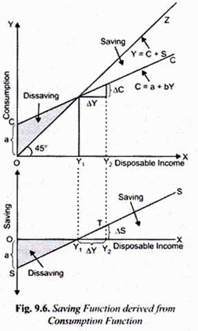
In Fig. 9.6 we have drawn the saving curve SS in the panel at the bottom. The saving curve SS shows the gap between consumption curve CC and the income curve OZ in the upper panel of Fig. 9.6.

It will be seen that up to income level OY₁ consumption exceeds income, that is, there is disserving. Beyond income level OY₁ there is positive saving. It is worth mentioning that as average propensity to consume (APC) falls with the increase in income in the upper panel, average propensity to save rises as income increases. Thus in Fig. 9.6 with the increase in income not only the absolute amount of saving increases, the average propensity to save also increases.

2. Marginal Propensity to Save (MPS):

Whereas average propensity to save indicates the proportion of income that is saved, marginal propensity to save represents how much of the additional disposable income is devoted to saving. The marginal propensity to save is therefore change in savings induced by a change in the disposable income.

Thus,

MPS = ∆S/ ∆Y

For example, if disposable income increases from Rs. 10,000 to Rs. 12,000 and this causes planned savings to increase by Rs. 500 crores, marginal propensity to save is:

MPS = 500/2000 = 1/4 = 0.25

Since the additional income is either consumed or saved, the sum of marginal propensity to consume and marginal propensity to save is equal to one.

MPC + MPS = 1

This can be mathematically proved as under

From C + 5 = Y, it follows that any change in income (∆K) must induce either change in consumption (∆C) or change in saving (∆S). Thus.

∆C + ∆S = ∆Y

Dividing both sides by AK we have

∆C/∆Y + ∆S/∆Y = ∆Y/∆Y = 1

The concept of marginal propensity to save is graphically shown at the bottom of Fig. 9.6. It will be seen from this figure that when disposable income increases from OY₁ (say f 10,000) to OY₁ (say Rs. 12,000), that is, ∆Y = Rs. 2000, the saving increases by Y₂T, (Rs. 500), that is, ∆S is Rs. 500. Thus marginal propensity to save (MPS) is

∆S/∆Y = 500/2000 = 1/4 = 0.25