
The CAPM was developed to explain how risky securities are priced in market and this was attributed to experts like Sharpe and Lintner. Markowitz Theory being more theoretical, CAPM aims at a more practical approach to stock valuation.
It is no doubt based on the mean-variance approach to risk for assessment of investment as developed by Markowitz. It explains the behavioural pattern of investors in building up portfolios.
The equation for the CAPM theory is-
RJ = Rf + BJ (RM – Rf)
ADVERTISEMENTS:
RJ is expected rate of return on security ‘J’; Rf is risk free return.
BJ is Beta coefficient — a risk measure for the non-diversifiable part of total Risk. RM is return on Market Portfolio and RM – Rf is the excess return for the extra risk.
Assumptions of CAPM:
The CAPM is based on certain assumptions some of which are common to CAPM and MPT. CAPM is in fact developed as part of MPT (Modern Portfolio Theory).
The assumptions are first set out below:
ADVERTISEMENTS:
(1) The investor aims at maximising the utility of his wealth, rather than the wealth or return. The difference between them is that individual preferences are taken into account in the utility concept. While some have preference for larger risk who will have increasing marginal utility for wealth, for others, with less preference for risk the incremental wealth will be less attractive if it is attached with more risk. Thus, the preference of investors for risk return will be taken into account in this model.
(2) Investors have similar expectations of Risk and Return. Without these consensus standards, the estimates of mean and variance may lead to different forecasts with the result that the efficient portfolio of each will be different from that of the others. There will be innumerable efficient frontiers, each dependent on the set of preferences of individuals for risk and return. If investors do not have similar expectations, there will be no homogeneity in their conception and no single efficient frontier line will apply to all.
This in turn will imply that the price of an asset, which is the best estimate of the present value of future returns will be different for different investors. This assumption is therefore unrealistic for application in the real world.
(3) Investors make investment decision on a rational basis, depending on their assessment of risk and return. Risk is measured by two factors, mean and variance. In the CAPM we assume that rational investors diversify away their diversifiable risk, namely, unsystematic risk and only systematic risk remains which varies with the Beta of the security. While some use the beta only, as a measure of risk, others use both Beta and variance of returns (total Risk) as the sources of reward or expected return.
ADVERTISEMENTS:
As these perceptions of risk and reward vary from individual to individual, under CAPM we get a series of efficient frontier lines while in the case of MPT, there will be a single efficient frontier line for the conception of risk and return expectation is assumed to be homogeneous in the latter.
(4) Investors will have free access to all available information at no cost and no loss of time. If the information is not the same for all, no common efficient frontier line can be drawn. Besides even if the information is not available at the same time different conclusions can be drawn regarding expected return and risk and no single price of the capital asset can be conceived.
(5) Investors should have identical time horizons which again is highly unrealistic. Investors have different time horizons and their estimates of stock value will therefore differ, even as the estimated earnings are the same per year. Continuous time models are sometimes used to get over the above difficulty or again one can approximate a single period model as a proxy to multi-period model on the assumption that returns are the same over time and time has no relevance to expected returns and that expected returns are again independent of the past and current information.
While the above assumptions are common to both CAPM and MPT, some assumptions are specific to CAPM. Thus, there is a risk free asset, which gives risk free return. Investors can borrow and lend unlimited amounts at the same price. This assumption of risk free asset transforms the curved efficient frontier line to a linear one. Risk can be reduced by adding a risk free asset, or borrowing at the risk free rate.
Besides, it is also necessary to assume in CAPM that total asset quantity is fixed and all assets are marketable and divisible. This assumption implies that the liquidity requirement of investors is ignored and there will be no new issues, which are both unrealistic.
After the brief review of the above assumption we can summarize the requirements for CAPM as follows:
“Risk is measured by variance of expected returns. There are two components of Risk — systematic (non-diversifiable) and unsystematic (diversifiable). For diversifiable risk, the investor makes a proper diversification to reduce the risk and for the non-diversifiable portion, he uses the relevant Beta measure to adjust to his requirement or preferences. Due to the possibility of risk free asset and lending and borrowing at the free rate, the investor has two components of the portfolio — risk free assets and the risky market assets. His total return is summation from the above two components.
Under CAPM, the equilibrium situation arises when all frictions, like taxes, divisibility transaction costs and different risk-free borrowing and lending rates are assumed away. Equilibrium will be brought about by changes in prices due to changes in demand and supply.
Capital Market Line (CML):
Figure below depicts the capital market line with riskless rate of return. Point P is the riskless interest rate. Preferred investments are plotted along the line PMZ, by combination of both risky assets and risk free asset along with the borrowing and lending. The slope of the PMZ is the measure of the reward for Risk taking. P is the risk free return, Em — T is the measure of the risk premium — a return for the risk taking. The reward for waiting is the risk less interest rate, OP, and second reward is the return per unit of risk borne measured by the slope ‘a’ of the PMZ line. The internal rate can be considered as price of time and the slope of capital market line as price of the risk.
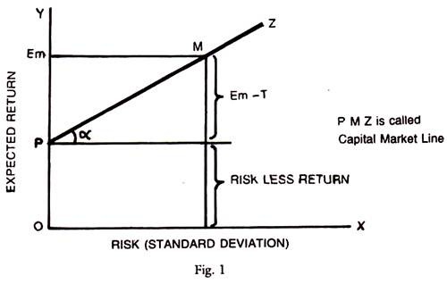
The equation of CML, connecting the risk less asset with the risky portfolio is-
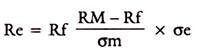
If the borrowing and lending rates are different, then O becomes the borrowing rate and OP will be the lending rate, as shown below.
The efficient frontier line with differential borrowing and lending rates will be as shown below:
ADVERTISEMENTS:
QMN is with the borrowing rate of OQ and PMN is with the lending rate of OP and ABC is the efficiency frontier line without borrowing and lending. The curved line will become linear; if once the riskless asset of borrowing and lending at fixed riskless rate is introduced.
The CML as described above reflects the relationship of total risk and expected return. Total risk includes both systematic and unsystematic risks. It may also include the risk free assets to reduce the total risk. The CAPM has two components of the capital market return, which are reward for waiting or riskless return, and the reward per unit of risk borne as measured by the slope of the CML line.
The investors will have their choice of efficient portfolio somewhere along the line of CML, as all efficient portfolios would be on it. Those which are less efficient will be below the line PMN, in the chart above. The internal rate can be thought as the price of time and the slope of the capital market line as the price of risk.
Security Market Line (SML):
ADVERTISEMENTS:
Unlike the CML, which considers the total risk as a measure of variability of returns, SML takes into account only the systematic risk, which is market related and is not possible to reduce or eliminate by diversification. Beta is the measure of risk of a security relative to the whole market, and is used in the SML.
Since the unsystematic risk is already taken care of by diversification in the construction of an efficient portfolio, it is desirable to develop an alternative to CML which will use Beta as the independent variable and can be adopted for use in portfolio management and in purchase of individual securities. Such a line is called Security Market Line, which depicts a linear relationship between expected return and the systematic risk.
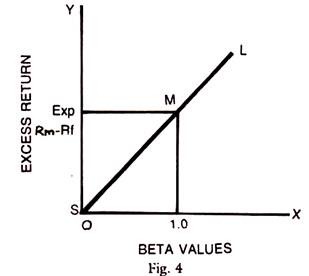
The SML curve drawn below shows a positive slope, indicating that the return and risk are positively related. The higher the risk the higher is the return. The Beta of Market portfolio, as represented by the BSE or NSE index is always one. But the company scrip can have Betas higher than 1 or lower than 1. Those with Beta’s less than 1 are defensive securities and those with Betas above 1 are called aggressive scrips. The graph below shows these types of scrips and the relationship of Beta to expected return.

SML is Security Market Line, OS is the risk-free return, OP is the return of the market, whose Beta is 1; those below Beta 1 are defensive and others are aggressive scrips in the market.
SML can be represented symbolically by an equation as-
ADVERTISEMENTS:
Ri = Rf + Bi (Rm – Rf)
Ri is the return on the security, i,
Rf is Risk-free return
Rm is Market Return.
Bi is Beta of Scrip i related to Market Risk.
If Rf = 10, Rm = 20, Bi = 1.5, which is more risky than the market average, then-
ADVERTISEMENTS:
Ri = 10 + 1.5 (20 – 10)
= 10 + 15 = 25.0% which is higher than the market return
Suppose the Bi is less risky than the market at 0.75 then Ri = 10 + 0.75 (20 – 10)
= 10 + 7.5 = 17.5%, which is lower than the market return
From the above equation, we can estimate the expected return on a security. It is represented as something like a premium or discount on the market return and can be compared. It can be a return on a security as distinguished from a portfolio.
If the security is correctly priced it will have Ri – Rf = 0 and SML curve goes through the origin Ri – Rf measures the excess return which varies with the risk taken. Within the chart it is seen that Rm – Rf is excess return if market Beta = 1. The security market line implies that the individual assets and portfolio should be on SML, if they are correctly priced. Beta values should then correctly represent the contribution to the risk of the security to the portfolio. All beta values assets lying above the SML are undervalued and those below the SML are overvalued. If we buy undervalued securities, the returns will be more and vice versa. It will thus be seen that SML curve assumes a critical importance in portfolio selection and individual investment decision.
CAPM Analysis:
The expected return of a portfolio in equilibrium is equal to risk free rate Rf, plus risk premium which is related to its Beta. Thus, Rp – Rf = risk premium and this is equal to BPM (Rm – Rf) where Rp is expected rate of return and Rf the risk free return.
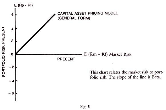
These symbols are the same as explained above. This leads us to the market model, which relates the expected excess return of the portfolio to the excess return of the market. This is an explanation of the risk premium which gives excess returns. The chart below presents the relation of E [(Rm) – (Rf)], to the E (RP – Rf), viz., in words, excess returns on a portfolio to the portfolio’s excess risk over the market risk. This chart presents CAPM in a general form with expected excess market risk related to expected excess return.
Market Model:
Risk Premium form is the one shown above and the equation for this is-
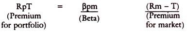
Beta relates the portfolio premium to market risk premium. If Beta is one they are the same.
ADVERTISEMENTS:
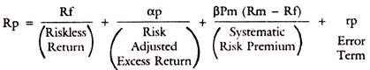
Market Model can be presented in the form of a regression equation. Taking the above equation for Risk premium of the portfolio, let us introduce a new concept of risk adjusted excess return which is generated by the expertise of the portfolio Manager, represented by the αp. This can be graphically represented as the y-axis intercept for the regression line, αp can be zero, positive or negative, depending on the performance of the portfolio.
When this model is presented in the Risk premium form, the equation is:
Rp – Rf = αp – Rf (1 – βpm) + β pm (Rm – Rf) + rp
αp° = αp -Rf(1 – βpm)
As the risk of the portfolio remains unaffected, βpm of the characteristic line remains unchanged but αp changes to αp° as follows:
αp° = αp – Rf (1 – βpm)
αp° is risk adjusted excess return.
αp is return on portfolio when the market return is zero. In other words, αp represents the excess return of the portfolio, when the market return is equal to riskless rate and rp is the error term or the residual.
αp° can be the same as αp, when Rf (1 – βpm) is zero which happens when βpm is 1; then the excess market return disappears. The above equation now becomes; Rp – Rf = αp 4- βpm (Rm – Rf) + rp
If error term is dropped then the equation becomes-
Rp = Rf + αP + βpm (Rm – Rf)
The above equation states that if the risk adjusted excess return on a portfolio is positive αp° > o, then the portfolio return is greater than what is normally expected, indicating superior return. If αp° is positive, the Portfolio Manager has shown his expertise in beating the market by showing return higher than the market return.
We have seen that the slope of SML curve is p. If we have a perfectly diversified portfolio in the CAPM, the error term disappears. If at the same time expected risk adjusted excess return αp0 of the portfolio is zero which is assured under Market Efficiency Theory, then the slope of the characteristic line is Beta of the portfolio. Thus, under condition of perfect markets, the slope of the Regression line is Beta and excess returns disappear (αp° = 0).
Uses and Limitations of CAPM:
In real world, investors get higher return for higher risk and they are more concerned with company related risks than with the market related risks, except in the case of trained investment analysts. Companies are found to use CAPM to determine the cost of equity for the firm, to estimate the required return for divisions or lines of business and to determine the hurdle rates for corporate investments and to evaluate the performance of investment Division in terms of costs and returns.
These hurdle rates of return are in general the required rates of return and the corporates assess the past performance of the costs and related returns for each of the Divisions. In the case of public utilities, the CAPM can be used to estimate the costs and rates to be charged to cover the costs. The CAPM is used to regulate the public utilities from the point of view of costs.
Historical return and Betas are used to select the proper risk in investments in the portfolio. CAPM is used to select securities, construct portfolios and evaluate the performance of the portfolio. It is thus a useful tool for investment analysis and portfolio management.
The limitations of the theory are also pointed out by many critics. This theory is unrealistic for any average investor, who goes by the fundamental factors influencing the company, its earnings, dividend and bonus record. Empirical tests of the Model have not proved very useful. The Model is built ex-ante factors while in reality the expectations of the future vary from person to person. Data and analysis is to be based on ex-post factors while anticipations of future risk and returns are ex- ante and both may not be related.
The CAPM is in fact not testable exactly as the exact composition of the market is known and is used in testing. The empirical tests conducted by Richard Roll and others were only tests on samples whether the proxy market portfolio was efficient or not. The use of surrogatives and proxies have not proved the theory as really useful and practical.
CAPM theory is thus a nice theoretical exposition but in actual world, it does not conform to the real world risk-return trends and empirical tests have not given unequivocal support to the theory. It is also found that there are many non-Beta factors influencing the returns. The calculation of Beta is itself of doubtful validity as the historical Betas may not reflect the future risks or returns. In the short-run in particular, projections on the basis of Betas on returns and risk have been found to be unreliable and results contrary to CAPM Theory were noticed. Thus, CAPM is a good theoretical tool but with its own limitations in practical applications.
Limitation of CAPM:
It is not realistic in the real world. This assumes that all investors are risk averse and higher the risk, the higher is the return. Investors ignore the transactions cost, information costs, brokerage taxes etc., and make decisions on the basis of single period horizon. The investors are given a choice on the basis of risk-return characteristics of an investment and they can buy at the going rate in the market. There are many buyers and sellers and the market is competitive and free forces of supply and demand determine the prices.
CAPM establishes a measure of risk premium and is measured by BJ (RM-Rf) Beta coefficient is the non-diversifiable risk of the asset, relative to the risk of the asset.
Suppose Tisco Company has a Beta equal to 1.5 and the risk free rate is say 6%. The required rate of return on the market (RM) is 15%.
Then, adopting the above equation, we have-
RJ = Rf + (BJ) (RM – Rf)
= 6 + 1.5 (15 – 6)
= 6 + 13.5 = 19.5%
If the market rate is 15% then the return on Tisco should be 19.5%, because the larger risk on Tisco than on the market.