Philips Curve (With Diagram)

Introduction:

A. W. Phillips, in his research paper published in 1958, indicated a negative statistical rela­tionship between the rate of change of money wage and the unemployment rate.

It was also shown that a similar negative relationship holds for rate of change of prices (i.e., infla­tion) and the unemployment level.

This rela­tion is usually generalised in the Phillips curve. Phillips first examined this negative relationship using data from the UK during the period 1861-1957.

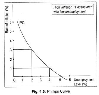
The Phillips curve, drawn in Fig. 4.5, shows that as the unemployment level rises, the rate of inflation falls. Zero rate of inflation can only be achieved with a high positive rate of un­employment of, say 5 p.c., or near full em­ployment situation can be attained only at the cost of high rate of inflation. Thus, there exists a trade-off between inflation and unemployment; the higher the inflation rate, the lower is the unemployment level.

This Phillips curve relation poses a di­lemma to the policymakers. If the objective of price stability is to be attained, the country must accept a high unemployment rate, or if the country designs to reduce unemployment, it will have to sacrifice the objective of price stability.

However, towards the end of the 1960s, the stable relationship between the two began to look unstable as unemployment, wages, price all began to rise. All these developments re­sulted in the emergence of newer theories and, hence, economic policies.

Meanwhile, the Phillips curve had been discredited although—in the 1960s and early 1970s economists attempted to explain infla­tion in terms of the logic of A.W. Phillips. Policymakers (both conservatives and liber­als) were a confused lot—what to choose: high rate of inflation and low unemployment or low rate of inflation coupled with high vol­ume of unemployment? Because of this con­fusion experienced by policymakers, econo­mists tried to find an alternative solution.

In fact, many authors came out and suggested that no longer i.e., in the 1970s and 1980s, the conclusion made by Phillips holds. It had been demonstrated by them that no particular re­lationship between inflation and unemploy­ment did exist. During the late 1970s and 1980s both inflation and unemployment changed but not in a direction suggested by Phillips for the previous 100 years (1861-1957).

This is means disappearance of trade-off between inflation and unemployment. Some authors then began to argue that no such stable relationship be­tween inflation and unemployment holds as shown in Fig. 4.5.

The Expectations-Augmented Phillips Curve:

Monetary economist Milton Friedman chal­lenged the concept of stable relationship be­tween inflation and unemployment rates as shown in Fig. 4.5. Friedman argues that such trade-off, i.e., negative relationship between inflation rate and unemployment—may hold in the short period, but not in the long run. Price or inflation expectations influence the Phillips curve.

In other words, Phillips curve shifts or changes its position as expectations regarding price level change. If people expect that inflation in the coming period will per­sist, the Phillips curve will shift to the right or if inflationary expectations show a downward trend, the Phillips curve will then shift its po­sition to the left.

In the short run, Phillips curve may shift either to the right, or to the left if the relationship between these variables—infla­tion rate and unemployment rate—is not sta­ble or inflationary expectations are stable. In other words, if inflationary expectations are deemed to be stable, then there would not be any shift in the Phillips curve as such.

Regarding the shifting of the Phillips curve, Friedman considers influence of inflationary expectations. This is called the theory of ‘adap­tive expectations’—expectations that are al­tered or ‘adopted’ to experienced events. In the short run, people make incorrect expecta­tions of the price changes because of incom­plete information. That is why a trade-off re­lationship emerges.

But in the long run, ac­tual and expected price changes become equal as expectations regarding price changes be­come equal when expectations regarding price changes tend to become rational. This rational expectations view suggest that people guess future economic events rather correctly in the long run.

Thus, the impact of expectations, whether adaptive or rational, have an impor­tant bearing on the relationship between in­flation and unemployment rates. It is because of expectation, Friedman argues that there is no trade- off between inflation and unemploy­ment in the long run.

Before we present Friedmanian long run Phillips curve in terms of a diagram, we must define the idea of ‘natural rate of unemploy­ment’ (NRU) which was introduced by Fried­man. Unemployment is ‘natural’ when some people either do not get jobs or are unwilling to accept jobs at the equilibrium real wage. Such a ‘natural’ rate of unemployment, may be considered as a situation of ‘full employ­ment’ of an economy.

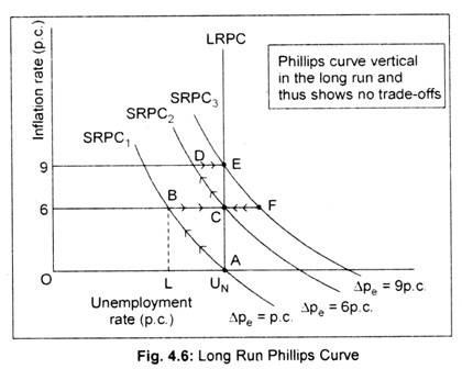
In Fig. 4.6 we have drawn the long run Phillips curve as a vertical line through the ‘natural rate of unemployment’. Further, we have drawn three short run Phillips curves (SRPC₁, SRPC₂ and SRPC₃) representing dif­ferent expected rates of inflation. The curve SRPC₁ shows ‘zero’ inflationary expectations (∆P_e = 0 p.c.) and a high rate of unemploy­ment or NRU, U_N. SRPC₂ shows a high ex­pected rate of inflation, say 6 p.c. (∆P_e= 6 p.c.). SRPC₃ shows more higher expected inflation rate, say 9 p.c. (∆P_e = 9 p.c.).

As people’s ex­pectation about future price level changes, short-run Phillips curve shifts upwards show­ing trade-offs between inflation and unem­ployment. Since, in the long run expected in­flation matches the actual inflation, the long run Phillips curve i.e., LRPC, becomes verti­cal at NRU or point U_N. It follows then that in the long run, there is no trade-off between the two.

In the long run, any positive rate of infla­tion may persist with a natural rate of unem­ployment or the non-accelerating inflation rate of unemployment (NAIRU) i.e., the rate of un­employment at which inflation is neither ac­celerating or decelerating.

We assume that the economy initially is at point A in Fig. 4.6 at the NRU, i.e., U_N with a zero actual and expected inflation rate. Fur­ther, we assume that the government thinks that this unemployment rate is pretty high and thus, takes step to reduce unemployment rate to OL. Adoption of policy measures say, ex­pansion in money supply causes aggregate demand to rise, and thus, wage rate to rise say by 6 p.c., and the level of unemployment to drop from OA to OL. This may cause a rise, say, 6 p.c. in the price level. The economy then moves from point A to B, thereby suggesting a higher inflation rate and a lower unemploy­ment rate along the SRPC₁.

Since workers expect price level to rise, the Phillips curve will shift upward to the right. Workers will now pitch a higher demand for wages and, as a consequence, a higher rate of inflation will appear at any given unemploy­ment rate.

If the same money wage growth is maintained, the economy will come back to U_N i.e., point A, but with an inflation rate of 6 p.c. This long run adjustment helps to move the economy from point B to point C. Further increase in money supply will result in tem­porary reductions in unemployment below the NRU, U_N (i.e., movement from point C to point D) but at a higher rate of inflation (say, 9 p.c.). The SRPC then shifts to SRPC₃, the economy in the long run moves from point D to E.

If the inflation rate is required to be low­ered down, policymakers will then be forced to increase the ‘natural’ rate of unemployment, beyond U_N. Then, based on a lower expected inflation rate, adjustment will take place along SRPC₃, from point E to F. As money wage de­clines more jobs will be available and unem­ployment rate will continue to fall until point C (i.e., natural unemployment rate, U_N) on SRPC₂ is reached. Thus, the LRPC is a vertical one through NRU, U_N, joining points A, C, E, and so on.