Short Run Equilibrium of a Firm under Perfect Competition | Markets

We shall now specifically discuss the ‘short-run’ equilibrium of a firm under perfect competition. We assume that the goal of the firm is to earn the maximum profit. Therefore, the point of profit maximisation is the firm’s equilibrium point. By the profit of the firm, we shall mean the profit in excess of normal profit which may also be called the pure profit or the economic profit.

We know that, in the short run, the firm may increase the quantity produced of its output (q) by increasing the use of the variable inputs. On the other hand, the firm may change, in the long run, the use of all the inputs, variable and fixed, by required amounts to increase its q.

That is why the short-run and long-run cost situations are not the same. The equilibrium of the firm in the short-run cost situation is called the short-run equilibrium and that in the long run cost situation is called the long-run equilibrium.

We shall discuss here the short-run equilibrium of a competitive firm. Let us suppose that the SAC and SMC curves of Fig. 10.5 are, respectively, the firm’s short-run average and marginal cost curves, and the AVC curve is its average variable cost curve.

All these three curves are U- shaped owing to the law of variable proportions (LVP). We may know what would be the firm’s average cost, marginal cost and average variable cost at any q, in the short run, from its SAC, SMC and AVC curves.

On the other hand, the AR and MR curves of the competitive firm would be identical and this curve would be the horizontal straight line at the level of the ruling market price (p) of the product. For example, in Fig. 10.5, when the price of the product is p₁, the firm’s AR = MR curve is the line AR₁ = MR₁. Here, at any q, the firm’s AR and MR, both, would be P₁ = constant.

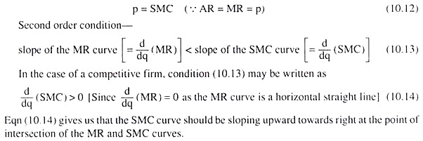
The short-run profit maximising or equilibrium conditions of the firm are

First order condition (FOC)—

MR = SMC                                              (10.11)

That is, FOC would be fulfilled at the point of intersection of the MR and SMC curves of the firm. In the case of a competitive firm, condition (10.11) may be written as

 

 

 

 

 

 

 

 

In Fig. 10.5, when the price of the product is p₁, the firm’s AR = MR curve is AR₁ = MR₁ and the firm’s short-run equilibrium point is E₁. At E₁, both the conditions (FOC and SOC) of firm’s equilibrium have been satisfied. For, first, E₁ is the point of intersection of the firm’s MR and SMC curves, i.e., at this point, we obtain MR = SMC, or, p = SMC (p = AR = MR).

That is, the FOC has been satisfied at the point. Second, at E₁ or at the MR = SMC point, the firm’s SMC curve is positively sloped, i.e., at E₁, the SOC of firm’s equilibrium has also been satisfied.

Therefore, at p = p₁ (or op₁), if the firm produces q = q₁ (or, oq₁ of output at the point E₁, then it would be in short-run profit-maximising equilibrium.

At E₁, we obtain the firm’s AR (= q₁E₁ = Op₁) > SAC (= q₁L₁)

⇒ AR x oq₁ > SAC x oq₁

⇒ TR (= □OP₁E₁q₁) > STC (= □OSL₁q₁)

Therefore, at E₁ the firm is earning a positive amount of excess profit or pure profit (re), since STC includes normal profit. The amount of the maximum π here is

π = TR – STC

= □OP₁E₁q₁ – □OSL₁q₁ = □SP₁E₁L₁

We may easily see now with the help of Fig. 10.5 that if the price of the product (p) diminishes, but yet is greater than p₃, then the firm’s equilibrium point would move down towards left along the firm’s SMC curve. As a result, the equilibrium output of the firm will diminish.

For example, at p = p₂ (< p₁), the firm’s equilibrium point would be E₂ on the SMC curve and its equilibrium output would be q₂ (< q₁). But at such a point (E₂), since AR (= p) is still greater than SAC (AR > SAC), the firm would still be able to earn a positive excess or pure profit, but the amount of profit here would be less than that obtained at E₁ (p₁, q₁).

This is because, as p diminishes (from p) to p₂), AR (= p) diminishes along the SMC curve from q₁E₁ to q₂E₂ and SAC diminishes along the SAC curve from q₁L₁ to q₂L₂.

Since the SMC curve is steeper than the SAC curve, the fall in AR is greater than the fall in SAC. As a result, the amount of pure profit per unit of output would be smaller (= E₂L₂) at E₂ than what it was at E₁ (= E₁L₁), and also output (q₂) is smaller at E₂ than what it was at E. So the total amount of pure profit at E₂ would be less than that at the point E₁.

The price p = p₃ in Fig. 10.5 is very important. For, if the firm sells q = q₃ at p = p₃, then it would be able to earn just the normal profit— the amount of excess or pure profit here would be zero. If the price is p₃, then the firm’s AR = MR line would be AR₃ = MR₃.

What is special about p = p₃ is that at this price, the firm’s AR₃ = MR₃ line touches the SAC curve at the latter’s minimum point E₃. (We may note here that a horizontal straight line like AR₃ = MR₃ may touch a U-shaped curve like SAC only at the latter’s minimum point.)

Now from the AC-MC relation, we know that, at the point E₃ (which is the minimum point of the SAC curve), the SMC curve intersects the SAC curve from below, and then goes above it. Therefore, the point E₃ lies on all the three curves, viz., AR₃ = MR₃, SAC and SMC. That is why at the point E₃, i.e., at p = p₃ and q = q₃, we obtain

p = AR = MR = SMC = SAC                                              (10.15)

Since, at the point E₃, the FOC of the firm’s equilibrium (MR = SMC) and the SOC (upward sloping SMC curve), both have been satisfied, this point (E₃) is the firm’s equilibrium or profit- maximising point. But, since at E₃, we have AR = SAC, or, TR = STC, the firm is able to earn only the normal profit at this point.

In other words, at the point E₃(p₃, q₃), the amount of maxi­mum profit that the firm would be able to earn is just equal to the normal profit, i.e., at the maximum profit point here, the amount of the firm’s excess profit or pure profit (n = TR – STC) would be equal to zero. That is why the point E₃ is called the break-even point at E₃, the firm’s total revenue (TR) and short-run total cost (STC) have broken even or have become equal.

Now, if the price of the product falls below the break-even price p₃, the firm would not be able to earn even the normal profit. Let us suppose that p falls from p₃ to p₄ in Fig. 10.5. Then the AR = MR line of the firm would shift downwards from AR₃ = MR₃ to AR₄ = MR₄ and the equilibrium point of the firm would be E₄(p₄, q₄).

Since AR₃ = MR₃ line just touched the SAC curve at the point E₃ and the AR₄ = MR₄ line lies below AR₃ = MR₃, it follows that the AR₄ = MR₄ line lies below the SAC curve throughout its length.

Therefore, at any output now, the firm’s AR would be less than its STC, and so, at the equilibrium point E₄(p₄, q₄), the firm’s pure profit π = TR – STC would be negative, i.e., the firm now would earn less than its normal profit, or, it has to bear some amount of loss which is equal to STC – TR.

In Fig. 10.5, at q = q₄, the firm’s (negative) profit per unit of output is

AR – SAC = q₄E₄ (= OP₄) – q₄ L₄

= – E₄L₄

and the total amount of (negative) profit is

π = q₄ x (AR – SAC)

= – q₄ x E₄ L₄ = negative

i.e., the total amount of loss here is equal to q₄ x E₄L₄.

Although, here, the firm has to bear a certain amount of loss, it cannot leave the industry in the short run, which it may do, however, in the long run. Of course, in the short run, the firm may shut down its production, i.e., it can reduce its production to zero, if it finds that this would help it to reduce its loss. Let us now see what the firm’s considerations are in this case.

In a situation of negative profit or positive loss, if the firm shuts down its production, then at q = 0, we would obtain, on the one hand, its TR to be zero, because the firm is selling nothing (TR = p x q = p x 0 = 0), and, on the other hand, the firm’s STC = TVC + TFC = 0 + TFC = TFC (since, in the short-run, at q = 0, TVC = 0). Therefore, at q = 0, we get the firm’s profit to be

π = TR – TVC – TFC

= 0 – 0 – TFC = – TFC

That is, in a situation of loss, if the firm shuts down production, then its profit will be negative, being equal to – TFC, and its loss will be equal to TFC = constant.

On the other hand, if, in such a situation, the firm continues production, then at q > 0, we would have TR > 0, TVC > 0, along with TFC > 0. If, here we have TR ≥ TVC, or, TR – TVC ≥ 0, then we would have n π ≥ -TFC i.e., the firm’s loss (which is here equal to |π|) will be less than, or, equal to TFC.

Therefore, in a situation of loss, when the firm’s goal of profit maximisation becomes the goal of loss minimisation, the firm will continue its production if it finds that at the concerned output level (like q = q₄ in Fig. 10.5), TR ≥ TVC, i.e., AR ≥ AVC [TR ≥ TVC => TR/q ≥ TVC/q => AR > AVC].

This may require a little more explanation.

In a situation of loss, the loss-minimising firm will continue production if p = AR > AVC; but, it will be indifferent between continuing and discontinuing production with the amount of loss being equal to TFC in both cases, if, p = AR = AVC.

However, in the p = AVC case, since the loss does not amount to more than TFC if the firm continuous production, we may assume that the firm will do so (rather than shutting down) if p = AVC. Or, we may take it in this way.

There must be a cut-off value of p which would separate the range of positive output from that of no output. Here p = AVC may be taken to be that cut-off value of p. If p > AVC, the firm will continue production and if p < AVC, the firm will shut down.

(It may be noted here that if p = AVC is taken to be the point at which the firm actually shuts down, then in the continuous case, determination of the said “cut-off value” of p becomes impossible.)

We may illustrate with the help of Fig. 10.5. Here, at p = p₅, the firm’s AR₅ = MR₅ line has touched its AVC curve at the latter’s minimum point E₅(p₅, q₅). As we know, the firm’s SMC curve also passes through this point.

That is why, at E₅, we obtain:

p = AR = MR = SMC = AVC (< SAC)                                       (10.16)

It is obvious from (10.16) that at E₅(p₅, q₅), AR < SAC implies a situation of loss, MR = SMC implies loss minimisation and p = AVC implies that the firm is on the verge of shutting down. That is why the point E₅ is called the shutdown point. We have to remember, however, that, at E₅, the firm will not actually shut down, but it is on the verge of shutting down.

The firm will actually shut down when p falls below p₅, for if p falls below p₅ to, say, p₆, the firm’s AR₆ = MR₆ line will lie below the AVC curve throughout its length, and we have p < AVC, whatever may be the firm’s output.

In Fig. 10.5, when p = p₆ < p₅, the firm’s AR = MR line intersects the SMC curve at the point E₆ (p₆, q₆), and, at this point, the SMC curve is upward sloping. So, at the point E₆, both the FOC and SOC of profit maximisation or loss minimisation have been satisfied.

However, at this point, E₆, or, at p = p₆, the firm will not produce any output, for if it produces an output of q = q₆, it would find:

p = AR = MR = SMC < AVC < SAC                                                 (10.17)

In (10.17), MR = SMC indicates that E₆ is a profit-maximising or loss-minimising point, and p < AVC indicates that, for loss minimisation, the firm would have to actually shut down its production, i.e., its short-run supply or q would be zero.

From the above analysis of the short-run equilibrium of a firm under perfect competition, we have seen that, in the short run, at the given price, the firm may produce and sell a positive quantity of output and, thereby, it may earn the maximum positive amount of pure profit, or, it may earn only the normal profit (pure profit = 0), or it may earn less than normal profit, i.e., it may suffer from negative pure profit or loss; or, at the given price, the firm may not sell any­thing at all. Everything depends on the ruling market price vis-a-vis the SAC and AVC at the firm’s equilibrium point.

From the Short-Run Equilibrium of the Firm to the Short-Run Supply Curve of the Firm:

The discussion of the short-run equilibrium of a competitive firm leads us to the concept of the short-run supply (SRS) curve of such a firm. Because, by definition, the SRS curve of a competitive firm gives us the equilibrium quantity of output supplied by the firm in the short run at any particular price of the product.

For example, as we have seen in Fig. 10.5, the equilibrium (p = SMC) quantity of output produced and supplied by the firm at p = p₁ is q = q₁.

Therefore, the short-run supply (SRS) of the firm at p = p₁ is q = q₁, and the point E₁ (p₁, q₁) on the SMC curve is also a point on the firm’s SRS curve. Again, if the price of the product diminishes from p, to p₂, the firm’s short-run equilibrium output or short-run supply (SRS) diminishes from q, to q₂ along the firm’s SMC curve.

Therefore, the point E₂(p₂, q₂) on the SMC curve is also a point on the firm’s SRS curve. Similarly, as the price diminishes from p₂ to p₃ to p₄ to p₅, the firm’s SRS diminishes along its SMC curve from q₂ to q₃ to q₄ to q₅, respectively, and the points E₃, E₄, and E₅ on the SMC curve are also points on the firm’s SRS curve.

Since the firm’s supply (SRS) changes with the price changes along its SMC curve and, as we have seen, the points on the SMC curve are also points on its SRS curve, the SMC curve itself (though not the whole of it) would be the firm’s SRS curve.

To be precise, the portion of the SMC curve that lies on or above the minimum point of the firm’s AVC curve would be its SRS curve. This is because, only for p > AVC, we obtain the firm’s supply to be positive. In Fig. 10.5, only for p > p₅, we obtain the SMC curve to be the firm’s SRS curve, giving us the positive quantity of output supplied by the firm at any price in this range, and the equation of this part of the firm’s SRS curve is

p = SMC(q), SMC’ > 0                                  (10.18)

We have also obtained already that for p < AVC, the firm’s output or SRS would be zero. Therefore, in Fig. 10.5, for p < p₅, the firm’s SRS curve would be the p-axis which is the vertical axis, and the equation of this part of the firm’s SRS curve is

q = 0                                                                (10.19)

Since there is a one-to-one relation between q and SMC, the inverse of (10.18) may better be taken as the equation of the firm’s SRS curve. This equation is

q = q (p), q’ > 0                                            (10.20)

where q is the quantity supplied in the short run at any p.

Accordingly, we have obtained the following in Fig. 10.5:

(i) For p > p₅, the SMC curve is the firm’s SRS curve. [eqns. (10.18), (10.20)]

(ii) For p < p₅, the p-axis or the vertical axis is the firm’s SRS curve. [eqn. (10.19)]

(iii) Therefore, at p = p₅, there is a discontinuity in the firm’s SRS curve, because, for p = p₅, the firm’s SRS is q₅ and, for p < p₅, the firm’s SRS is zero. So there can be no output of the firm between zero and q₅.

(iv) The Firm’s SRS Curve is Obtained in Two Parts:

One part is given by (i) above and the other part is given by (ii) above. In between the two parts, there is a discontinuity like the one shown by the broken line at p = p₅ in Fig. 10.5. The short-run supply curve of a competitive firm in two parts, along with the discontinuity, has been reproduced from Fig. 10.5 in Fig. 10.6(a).

From the Short-Run Supply of a Firm to the Short-Run Supply of the Industry:

By the short-run supply (SRS) of a perfectly competitive industry, we mean the quantity supplied by all the firms in the industry at any particular price. That is why the SRS curve of the industry is the horizontal or lateral summation of the SRS curves of all the firms in the industry.

The SRS of the industry at any particular price is obtained from the SRS curve of the industry in the same way as the SRS of a firm is obtained from the SRS curve of the firm. We may illustrate the process of obtaining the SRS curve of the industry as a horizontal summation of the SRS curves of the firms with the help of Fig. 10.6.

To make our job simple, we shall assume here:

(i) that the number of firms in the industry is only two, and

(ii) the two firms are equal in respect of their cost.

In Fig. 10.6 (a), we have shown firm A’s SRS curve, viz., SRS_a, and in Fig. 10.6 (b), we have shown firm B’s SRS curve, viz., SRS_B.

In these figures, we have assumed that the price p* (or, Op*) is equal to minimum AVC. Therefore, at p < p*, the quantities produced and sold, i.e., the quantities supplied of both the firms, would be equal to zero, i.e., the SRS curve of each of these firms would be the op* segment of its p-axis. But if p > p*, the supply of both the firms would be positive and their SRS curves would be sloping upward towards right.

In Fig. 10.6(c), we have shown the industry’s SRS curve, and it has been obtained as the horizontal summation of the SRS_A and SRS_B curves. Since the quantity supplied by each firm would be zero at any p < p*, the industry’s supply for p < p* would also be zero.

That is, for p < p*, the SRS curve of the industry would be the op* segment of the p-axis of Fig. 10.6(c). The equation of this part of the SRS curve of the industry would be

q = 0                                                     (10.21)

where q is the quantity supplied by the industry.

On the other hand, for p > p*, the SRS curves of the firms would be sloping upward towards right and so the industry’s SRS curve, which is the horizontal summation of the firms’ SRS curves, would also be sloping upward towards right. The equation of this part of the industry’s SRS curve would be

 

 

 

 

 

 

 

 

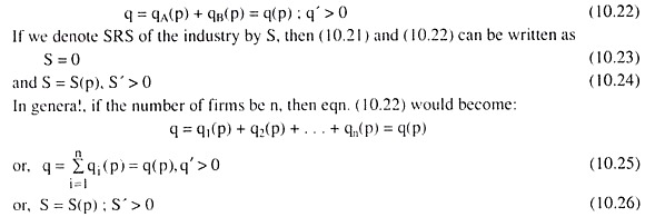
We have seen in the above discussion that, like the SRS curve of the firm, the SRS curve of the industry has also two parts—one of them is a vertical straight line and its equation is (10.23), and the other part is upward sloping towards right, and its equation is (10.24) or (10.26).

We have to note that, like the firm’s SRS curve, the industry’s SRS curve also has a discontinuity. This discontinuity has been indicated in Fig. 10.6(c) by a broken line.