Price Determination under Perfect Competition | Markets | Economics

Perfect competition is defined as a market situation where there are a large number of sellers of a homogeneous product. An individual firm supplies a very small portion of the total output and is not powerful enough to exert an influence on the market price.

A single buyer, however large, is not in a position to influence the market price. Market price in a perfectly competitive market is determined by the interaction of the forces of market demand and market supply. Market demand means the sum of the quantity demanded by individual buyers at different prices.

Similarly, market supply is the sum of quantity supplied by the individual firms in the industry. Each seller and buyer takes the price as determined. Therefore, in a perfectly competitive market, the main problem for a profit-maximizing firm is not to determine the price of its product but to adjust its output to the market price so that profit is maximized.

Price determination under perfect competition is analyzed under three different time periods:

(a) Market Period

(b) Short Run

(c) Long Run

(a) Market Period:

In a market period, the time span is so short that no firm can increase its output. The total stock of the commodity in the market is limited. The market period may be an hour, a day or a few days or even a few weeks depending upon the nature of the product.

For example, in the case of perishable commodities like vegetables, fish, eggs, the period may be a day. Since the supply of perishable commodities is limited by the quantity available or stock in day that neither can be increased nor can be withdrawn for the next period, the whole of it must be sold away on the same day, whatever may be the price.

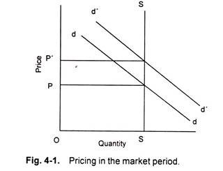
Fig 4.1 shows that the supply curve of perishable commodities like fish is perfectly inelastic and assumes the form of a vertical straight line SS. Let us suppose that the demand curve for fish is given by dd. Demand curve and supply curve intersect each other at point R, determining the price OP. If the demand for fish increases suddenly, shifting the demand curve upwards to d’d’.

The equilibrium point shift from R to R” and the price rises to OP’. In this situation, price is determined solely by the demand condition that is an active agent.

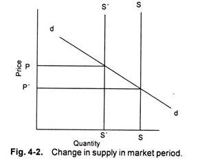
Similarly, if the demand for a product is given, as shown in demand curve SS in figure 4.2. If the supply of the product decreases suddenly from SS to S’S’, the price increases from P to P’. In this case price is determined by supply, the supply being an active agent.

In this case supply curve shifts leftward causing increase in price of the reduced supply goods. Given the demand curve dd and supply curve SS, the price is determined at OP. Demand curve remaining the same, the decrease in supply shifts the supply curve to its left to S’S’. Consequently, the price rises from OP to OP’.

The supply curve of non-perishable but reproducible goods will not be a vertical straight line throughout its length. This is for certain goods can be withdrawn from the market if the price is too low as the seller would not sell any amount of the commodity in the present market period and would like to hold back the whole stock.

The price below which the seller declines to offer for any amount of his product is known as ‘reserve price’. Thus, the seller faces two extreme price-levels; at one he is ready to sell the whole stock and the other he refuses to sell any. The amount he offers for sale will vary with price.

The seller will be ready to supply more at a higher price rather than at a lower one will depend upon his anticipations of future price and intensity of his need for cash. The supply curve of a seller will, therefore, slope upwards to the right up to the price at which he is ready to sell the whole stock. Beyond this point, the supply curve will become a vertical straight line whatever the price.

(b) Pricing in the Short Run- Equilibrium of the Firm:

Short period is the span of time so short that existing plants cannot be extended and new plants cannot be erected to meet increased demand. However, the time is adequate enough for producers to adjust to some extent their output to the increase in demand by overworking their fixed capacity plants. In the short run, therefore, supply curve is elastic.

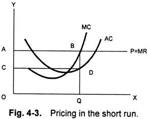
Figure 4.3 shows the average and marginal cost curves of the firm together with its demand curve. Demand curve, in a perfectly competitive market, is also the average revenue curve and the marginal revenue curve of the firm. The marginal cost intersects the average cost at its minimum point. The U-shape of both the cost curves reflects the law of variable proportions operative in the short run during which the size of the plant remains fixed.

The firm is in equilibrium at the point B where the marginal cost curve intersects the marginal revenue curve from below:

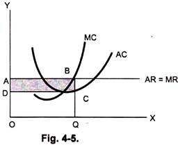
The firm supplies OQ output. The QC is the average cost and the firm earns total profit equal to the area shown by ABCD. The firm maximizes its profit. Earlier to the point of equilibrium, the firm does not attain the maximum profit as each additional unit of output brings more revenue that its cost. Any level of output greater than OQ brings less marginal revenue than marginal cost.

For the equilibrium of a firm the two conditions must be fulfilled:

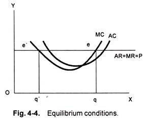
(a) The marginal cost must be equal to the marginal revenue. However, this condition is not sufficient, since it may be fulfilled and yet the firm may not be in equilibrium. Figure 4.4 shows that marginal cost is equal to marginal revenue at point e’, yet the firm is not in equilibrium as Oq output is greater than Oq’.

(b) The second and necessary condition for equilibrium requires that the marginal cost curve cuts the marginal revenue curve from below i.e. the marginal cost curve be rising at the point of intersection with the marginal revenue curve.

Thus, a perfectly competitive firm will adjust its output at the point where its marginal cost is equal to marginal revenue or price, and marginal cost curve cuts the marginal revenue curve from below.

The fact that a firm is in equilibrium does not imply that it necessarily earns supernormal profits. In the short-run equilibrium firms may earn supernormal profits, normal profits or may incur losses.

Whether the firm makes supernormal profits, normal profits or incurs losses depends on the level of the average cost at the short run equilibrium. If the average cost is below the average revenue, the firm earns supernormal profits. Figure 4.5 illustrates that the average cost QC is less than average revenue QB, and the firm earns profits equal to the area ABCD.

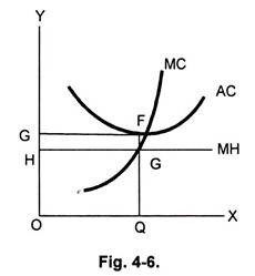
If the average cost is above the average revenue the firm makes a loss. Figure 4.6 shows that the Average cost QF is higher than QG average revenue and the firm is incurring loss equal to the shaded area EFGH. In this case the firm will continue to produce only if it is able to cover its variable costs.

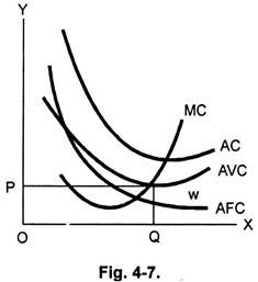
Otherwise it will close down, since by discontinuing its operations the firm is better off; it minimizes its losses. The point at which the firm covers its variable costs is called ‘the closing-down point’. If the price falls below or average costs rise, the firm does not cover its variable costs and is better off if it closes down. Figure 4.7 explains shut- down point.

Equilibrium of the Industry:

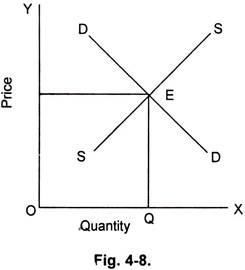
An industry is in equilibrium at that price at which the quantity demand is equal to the quantity supplied.

Figure 4.8 explains that DD is the industry demand and SS the industry supply. The point E at which industry demand and industry supply equalizes, the price OP is determined. OQ is the quantity demanded and quantity supplied. This, however, is a short run equilibrium where at the market-determined price some firms may be making supernormal profits, normal profits or making losses. In the long run the firms may not continue incurring losses. Loss making firms that cannot adjust their plant will close down.

Firms that are making supernormal profits will expand their capacity. Simultaneously new firms will be attracted into the industry. Free movement of firms in and outside the industry and readjustment of the existing firms in the industry will establish a long run equilibrium in which firms will just be earning normal profits and there will be no tendency of entry or exit from the industry.

(c) Pricing in the Long Run:

The long run is a period of time long enough to permit changes in the variable as well as in the fixed factors. In the long run, accordingly, all factors are variable and non- fixed. Thus, in the long run, firms can change their output by increasing their fixed equipment. They can enlarge the old plants or replace them by new plants or add new plants.

Moreover, in the long run, new firms can also enter the industry. On the contrary, if the situation so demands, in the long run, firms can diminish their fixed equipments by allowing them to wear out without replacement and the existing firm can leave the industry.

Thus, the long run equilibrium will refer to a situation where free and full scope for adjustment has been allowed to economic forces. In the long run, it is the long run average and marginal cost curves, which are relevant for making output decisions. Further, in the long run, average variable cost is of no particular relevance. The average total cost is of determining importance, since in the long run all costs are variable and none fixed.

In the short run a firm under perfect competition is in equilibrium at that output at which marginal cost equals price or Marginal Revenue. This is equally valid in the long run. But, in the long run for a perfectly competition firm to be in equilibrium, besides marginal cost being equal to price, price must also be equal to average cost. If the price is greater than the average cost, the firms will be making supernormal profits.

Lured by these supernormal profits, new firms will enter the industry and these extra profits will be competed away. When the new firms enter the industry, the supply or output of the industry will increase and hence the price of the output will be forced down. The new firms will keep coming into the industry until the price is depressed down to average cost, and all firms are earning only normal profits.

On the other hand, if the price happens to be below the average cost, the firms will be incurring loses. Some of the existing firms will quit the industry. As a result, the output of the industry will decrease and the price will rise to equal the average cost so that the firms remaining in the industry are making normal profits. Hence, in the long run, firms need not be forced to produce at a loss since they can leave the industry, if they are having losses. Thus, for a perfectly competitive firm to be in equilibrium in the long run, price must equal marginal and average cost.

Now when average cost curve is falling, marginal cost curve is below it, and when average cost curve is rising, marginal cost curve must be above it. Hence, marginal cost can be equal to the average cost only at the point where average cost curve is neither falling nor rising, i.e. at the minimum point of average cost curve. Therefore, it is at the point of minimum average cost curve, and the two are equal there.

Thus, the conditions for long run equilibrium of perfectly competitive firm can be written as:

Price = Marginal Cost = Minimum Average Cost.

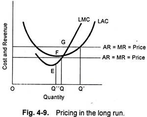
The conditions for the long run equilibrium of the firm under perfect competition can be easily understood from the Fig. 4.9, where LAC is the long run average cost curve and LMC in the long run marginal cost curve. The firm under perfect competition cannot be in long run equilibrium at price OP’, because though the price OP’ equals MC at G (i.e., at output OQ) but it is greater than the average cost at this output and, therefore, the firm will be earning supernormal profits.

Since all the firms are assumed to be identical, all would be earning supernormal profits. Hence, there will be attraction for the new firms to enter the industry. As a result, the price will be forced down to the level Op at which price, the firm is in equilibrium at F and is producing OQ” output.

At point F or equilibrium output OQ”, the price is equal to average cost, and hence the firm will be earning only normal profits. Therefore, at price OP, there will be no tendency for the outside firms to enter the industry. Hence, the firm will be in equilibrium at OP price and OQ output.

On the contrary, a firm under perfect competition cannot be in the long run equilibrium at price OP”. Though price OP” is equal to marginal cost at point E, or at output OQ” but price OP” is lower than the average cost at this point and thus the firm will be incurring losses.

Since all the firms in the industry are identical in respect of cost curves, all would be incurring losses. To avoid these losses, some of the firm will leave the industry. As a result, the price will rise to OP, where again all firms are making normal profits. When the price OP is reached, the firms would have no further tendency to quit.

Thus, to conclude that at price OP, the firm under perfect competition is in equilibrium in the long run when:

Price = MC = Minimum AC

Now, at price OP, besides all firms being in equilibrium at output OQ, the industry will also be in equilibrium, since there will be no tendency for new firms to enter or the existing firms to leave the industry, because all will be earning normal profits. Thus, at OP price, full equilibrium, i.e. equilibrium of all the individual firms and also of the industry, as a whole, is achieved in the long run under perfect competition.