How does an Individual Firm Reach Equilibrium?

The following article will guide you about how an individual firm reaches equilibrium under perfect competition.

Short Run:

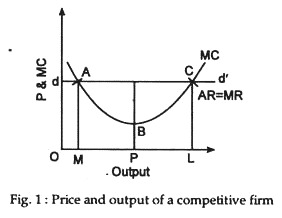
Under perfect competition the marginal revenue is equal to price. So the formula MR=MC becomes P=MC. The individual firm, under perfect competition, maximises its net revenue by fixing output at the point where its marginal cost is equal to the market price of the product.

If the marginal cost is less than the price, the firm gains by expanding output, if the marginal cost is higher than the price, the firm incurs losses and must reduce its marginal cost by reducing output. If it cannot do so, it must abandon production.

Under perfect competition, the individual firm cannot influence the price. It must take the average revenue (its demand) curve for granted and adjust its output according to its marginal cost curve.

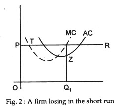
The short-run equilibrium position of a firm under perfect competition is illustrated in Fig. 2, where

OP = Price.

PR = Average Revenue Curve.

AC = Average Cost Curve.

MC = Marginal Cost Curve.

When output is OQ₁ the marginal cost is the same as the price. There­fore, the firm will produce OQ and sell it at price OP (=EQ).

In Fig. 1 the firm’s average cost (=Q₁Z) is less than the price (=EQ₁). Therefore, the firm is earning excess profits (=EZ per unit). In the long run there will be new entry and the excess profits will be competed away.

A diagram similar to this may be drawn in such a way as to make EZ negative. Such a diagram will illustrate the case where a firm is losing in the short run. In such cases the long period adjustment will take place by the exit of firms.

The result of ‘bad times’. In the long run the total revenue of the firm must cover both variable costs and fixed costs. In the short run, however, a firm may continue to produce if its variable costs are covered. This happens during ‘bad times’ if the firm expects that the situation will improve in the future. Rather than closing down its business, which will involve greater loss, the firm may carry on for some time at a small loss. This may be regarded as a method of minimising the loss.

Long Run:

In the long run, the total revenue of the firm must equal its total cost of production. (By definition, “total cost” includes normal profits). If the total revenue is greater than its total cost, the firm is making excess profits. Whenever there is excess profit, new firms will be attracted into the industry, the total output of the industry will increase and the price will fall.

The process will go on until the whole of excess profit is wiped out. If the total revenue is less than its total cost, the whole process of adjustment will be reversed. There will occur exit of firms, reduction in total output, and rise of prices. Finally at equilibrium, total revenue must equal total cost.

When total revenue equals total cost, the average revenue (or price) must equal average cost. This follows from the definition of the terms.

Let ‘q’ be the output, ‘p’ the price and V the average cost.

Then, total revenue = pq and total cost = aq.

At equilibrium, pq = aq. p=a.

For equilibrium, another condition also must be satisfied, viz., the mar­ginal revenue (or price) must equal the marginal cost. This is a general condition which determines at what level of output the net revenue, i.e., the difference between TR and TC is maximised.

For long-run equilibrium un­der perfect competition we thus get two necessary conditions:

1. Price = Marginal Cost

2. Price = Average Cost

Or, Price = Average Cost = Marginal Cost (by combining 1 and 2)

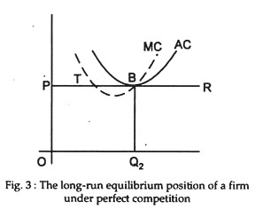
The long-run equilibrium po­sition of a firm under perfect competition is illustrated in Fig. 3.

Where,

OP = Price.

PR = Average Revenue.

AC = Average Cost Curve.

MC = Marginal Cost Curve.

OQ₂ = The equilibrium output.

When OQ₂ is the output, the price (OP) = (QB) = marginal cost (QB) = average cost (QB). Thus, all the equalities held in the long run.

The minimum average cost:

The horizontal line PR is the average reve­nue (demand) curve of the firm. In long-run equilibrium this curve is a tangent to the average cost curve, (otherwise there cannot be equality between price, average cost and marginal cost). Since PR is a horizontal line and AC is U-shaped, PR can be tangent to AC only at the lowest point of the latter. This means that in the long run under perfect competition the individual firm produces at the lowest possible average cost.

Other conditions:

Certain other conditions must also be fulfilled before a firm is in equilibrium.

They are stated below:

1. In Figures 2 and 3, it will be observed that the marginal cost curve cuts the marginal revenue curve at two points, viz., T and B. At both these points, MR=MC. But, the output indicated by the first point T is not an equilibrium output, because when output is increased beyond point T marginal cost is reduced and total revenue increases.

Here T is the point of minimum net revenue and not the maximum net revenue. From this we can come to the conclusion that at the point of equilibrium the marginal cost curve must cut the marginal revenue curve from below, i.e., the relative position of the two curves must be such that to the left of the equilibrium point marginal cost is less than marginal revenue, and to the right of the equilibrium point marginal cost is greater than marginal revenue.

2. In long-run equilibrium the firm must be earning not only the maxi­mum possible profit as is considered to be reasonable and usual in that line of business. If less than normal profit is earned some firms will go out of the industry. If more than normal profit is earned some new firms will join the industry.

In either case there will be changes in price and output. Hence, in long-run equilibrium each firm must be earning normal profit. This condition is fulfilled when the average cost curve of each firm belonging to the industry is tangent to its average revenue curve.

Equilibrium under different cost conditions:

The cost conditions of different firms are different.

It is possible to distin­guish between three possible cases:

(a) Where all factors are homogeneous:

This means that there is perfect competition in the factors’ market, all factors are identical, all factors are easily available and factor prices are constant. In this situation all firms have identical cost curves. The equilibrium positions are as shown in Figures 2 and 3. In the long run all firms earn normal profits although in the short run there may be super normal profits or losses.

(b) Where all factors, except entrepreneurs, are homogeneous:

This means that the entrepreneurs have different capacity (are ‘heterogeneous’) while all other factors are homogeneous. In this situation different firms have different cost curves. Some firms earn more than others, even in the long run. Earnings which are due to the superior ability of a particular entrepreneur cannot be competed away, even in the long run. They are analogous to rent.

(c) Where all factors are heterogeneous:

In this case the earnings of the different firms differ to a greater extent. Some firms earn supernormal profits.