Cournot’s Duopoly Model (With Diagram)

The earliest duopoly model was developed in 1838 by the French economist Augustin Cournot. The model may be presented in many ways.

The original version is quite limited in that it makes the assumption that the duopolists have identical products and identical costs.

Actually Cournot illustrated his model with the example of two firms each owning a spring of mineral water, which is produced at zero costs. We will present briefly this version, and then we will generalize its presentation by using the reaction curves approach.

Cournot assumed that there are two firms each owning a mineral well, and operating with zero costs. They sell their output in a market with a straight-line demand curve. Each firm acts on the assumption that its competitor will not change its output, and decides its own output so as to maximize profit.

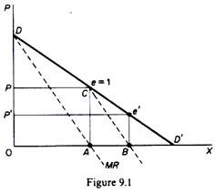
Assume that firm A is the first to start producing and selling mineral water. It will produce quantity A, at price P where profits are at a maximum (figure 9.1), because at this point MC — MR = 0. The elasticity of market demand at this level of output is equal to unity and the total revenue of the firm is a maximum. With zero costs, maximum R implies maximum profits, Π. Now firm B assumes that A will keep its output fixed (at 0/1), and hence considers that its own demand curve is CD’.

Clearly firm B will produce half the quantity AD’, because (under the Cournot assumption of fixed output of the rival) at this level (AB) of output (and at price F) its revenue and profit is at a maxi­mum. B produces half of the market which has not been supplied by A, that is, B’s output is ¼ (= ½. ½) of the total market.

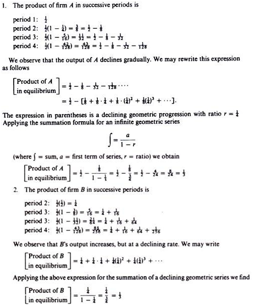
Firm A, faced with this situation, assumes that B will retain his quantity constant in the next period. So he will produce one-half of the market which is not supplied by B. Since B covers one-quarter of the market, A will, in the next period, produce ½(1 – ¼) = ½. ¾ = ⅜ of the total market.

Firm B reacts on the Cournot assumption, and will produce one-half of the unsupplied section of the market, i.e. ½ (1 – ⅜) = 5/16.

In the third period firm A will continue to assume that B will not change its quantity, and thus will produce one-half of the remainder of the market, i.e. ½ (1 – 5/16).

This action-reaction pattern continues, since firms have the naive behaviour of never learning from past patterns of reaction of their rival. However, eventually an equilibrium will be reached in which each firm produces one-third of the total market. Together they cover two-thirds of the total market. Each firm maximises its profit in each period, but the industry profits are not maximised.

That is, the firms would have higher joint profits if they recognised their interdependence, after their failure in forecasting the correct reaction of their rival. Recognition of their interdependence (or open collusion) would lead them to act as ‘a monopolist,’ producing one-half of the total market output, selling it at the profit-maximising price P, and sharing the market equally, that is, each producing one-quarter of the total market (instead of one-third).

The equilibrium of the Cournot firms may be obtained as follows:

Thus the Cournot solution is stable. Each firm supplies 4 of the market, at a common price which is lower than the monopoly price, but above the pure competitive price (which is zero in the Cournot example of costless production). It can be shown that if there are three firms in the industry, each will produce one-quarter of the market and all of them together will supply ¾ ( = ¼ . 3) of the entire market OD’.

And, in general, if there are n firms in the industry each will provide n /(n + 1) of the market, and the industry output will be n/(n + 1) = 1 /(n + 1) . n. Clearly as more firms are assumed to exist in the industry, the higher the total quantity supplied and hence the lower the price. The larger the number of firms the closer is output and price to the competitive level.

Cournot’s model leads to a stable equilibrium. However, his model may be criticized on several accounts

The behavioural pattern of firms is naive. Firms do not learn from past miscalcula­tions of competitors’ reactions.

Although the quantity produced by the competitors is at each stage assumed constant, a quantity competition emerges which drives P down, towards the competitive level.

The model can be extended to any number of firms. However, it is a ‘closed’ model, in that entry is not allowed: the number of firms that are assumed in the first period remains the same throughout the adjustment process.

The model does not say how long the adjustment period will be.

The assumption of costless production is unrealistic. However, it can be relaxed without impairing the validity of the model. This is done in the subsequent presentation of the model, based on the reaction-curves approach.

The reaction-curves approach is a more powerful method of analysis of oligopolistic markets, because it allows the relaxation of the assumption of identical costs and identical demands. This approach is based on Stackelberg’s indifference-curve analysis, which introduces the concept of isoprofit curves of competitors. We will first establish the shape of the isoprofit curves for substitute commodities, and from these curves we will subsequently derive the reaction curves of the Cournot duopolists.

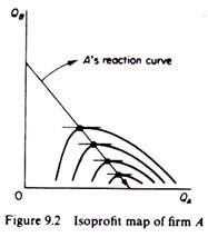
An isoprofit curve for firm A is the locus of points defined by different levels of output of A and his rival B, which yield to A the same level of profit (figure 9.2).

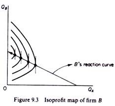
Similarly, an isoprofit curve for firm B is the locus of points of different levels of output of the two competitors which yield to B the same level of profit (figure 9.3).

From the above definitions it should be clear that the isoprofit curves are a type of indifference curves.

There is a whole family of isoprofit curves for each firm which have the following properties:

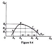
1. Isoprofit curves for substitute commodities are concave to the axes along which we measure the output of the rival firms. For example, an isoprofit curve of firm A is concave to the horizontal axis Q_A. This shape shows how A can react to B’s output decisions so as to retain a given level of profit. For example, consider the isoprofit curve Π_A1 in figure 9.4.

Suppose that firm B decides to produce the level of output B₁. A line parallel to the horizontal axis through B₁ intersects the isoprofit curve Π_A1 at points h and g. This shows that given the output that B decides to produce, firm A will realise the profit Π_A1 if it produces either of the two levels of output corresponding to points h and g, that is, either A_h or A_g. Assume that firm A decides to react by producing the higher level A_g.

If now firm B increases its output (say at the level B₂), firm A must decrease its output (at A_f) if it wants to retain its profit at the same level (Π_A1). If firm A continued to produce A_g while B increased its production, the total quantity supplied in the market would depress the price, and hence the profit of firm A would decline. Up to a certain point (e in figure 9.4) firm A must react to increases in B’s output by reducing its own production, otherwise the market price would fall and A’s profit would decrease. As firm A reduces its output, its costs also change, but the net profit (Π = R – C) remains at the same level (Π_A1), because of market elasticity and/or decreasing costs arising from a better utilisation of A’s plant.

Consider now point h. If firm A reacts to B’s initial decision by producing the lower output A_h, it will clearly earn the same profit Π_A1. If firm B decides to increase its output (at the levels B₂, B₃ and so on, up to B_e), firm A will react by increasing its output as well y4’s profit will remain the same despite the resulting fall in the market price, because of market elasticity and/or decrease in its costs due to a better utilisation of its plant.

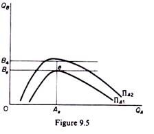
2. The farther the isoprofit curves (for substitute commodities) lie from the axes, the lower is the profit. And vice versa, the closer to the quantity-axis an isoprofit curve lies, the higher the profitability of the firm is. Consider figure 9.5. If firm B were to increase its output beyond B_e, firm A would not be able to retain its level of profit. Suppose that firm B decides to produce B₄. Firm A can react in three ways: increase, decrease or retain its output constant (at A_e). If A retains its output constant while B increases its production, the ensuing fall in the market price will result in a reduction in the revenue and in the profits of A, given its costs.

If firm A were to increase output beyond A_e, its profit would fall because of inelasticity of demand and/or increasing costs. If firm A were to reduce output below A_e, its profit would fall because of elasticity of demand and/or increasing costs. Thus firm A will earn a lower level of profit, no matter what its reaction, if B increased its output beyond B_e. A line through B₄ parallel to the Q_A-axis lies above Π_A1, and will intersect (or will be tangent) to an isoprofit curve which represents a lower profit for firm A.

In figure 9.5 the isoprofit curve Π_A2 represents a lower profit than Π_A1. To summaries for any given output that firm B may produce, there will be a unique level of output for firm A which maximises the latter’s profit. This unique profit-maximizing level of output will be determined by the point of tangency of the line through the given output of firm B and the lowest attainable iso­profit curve of firm A. In other words, the profit-maximising output of A (for any given quantity of B) is established at the highest point on the lowest attainable isoprofit curve of A.

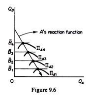
3. For firm A, the highest points of successive isoprofit curves lie to the left of each other. If we join the highest points of the isoprofit curves we obtain firm A’s reaction curve. Thus, the reaction curve of firm A is the locus of points of highest profits that firm A can attain, given the level of output of rival B. It is called ‘reaction curve’ because it shows how firm A will determine its output as a reaction to B’s decision to produce a certain level of output, A’s reaction curve is shown in figure 9.6.

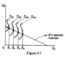
B’s isoprofit curves are concave to the Q_B axis. Their shape and position are deter­mined by the same factors as the ones underlying firm A’s isoprofit curves. The highest point of the isoprofit curves of B lie to the right of each other as we move to curves further away from the Q_B axis. If we join these highest points we obtain B’s reaction function (figure 9.7). Each point of the reaction curve shows how much output B must produce in order to maximize its own profit, given the level of output of its rival.

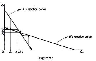
Cournot’s equilibrium is determined by the intersection of the two reaction curves. It is a stable equilibrium, provided that A’s reaction curve is steeper than B’s reaction curve. (This condition is satisfied by the assumption we made that the highest points of successive isoprofit curves of A lie to the left of one another, while the highest points of B’s isoprofit curves lie to the right of each other.) To see that, let us examine the situation arising from A’s decision to produce quantity A₁, lower than the equilibrium quantity A_e (figure 9.8). Firm B will react by producing B₁ given the Cournot assumption that firm A will keep its quantity fixed at A₁.

However, A reacts by producing a higher quantity, of A₂, on the assumption that B will stay at the level B₁. Now firm B, reacts by reducing its quantity at B₂. This adjustment will continue until point e is reached. The same equilibrium would be reached if we started from a point to the right of e. Thus e is a stable equilibrium.

Note that at point e each firm maximises its own profit, but the industry (joint profit) is not maximized (figure 9.9). This is easily seen by a curve similar to Edge-worth’s contract curve which traces points of tangency of the two firms’ isoprofit curves. Points on the contract curve are optimal in the sense that points off this curve imply a lower profit for one or both firms, that is, less industry profits as compared to points on the curve. Point e is a suboptimal point, and total industry profits would be higher if firms moved away from it on any point between a and b on the contract curve at point a firm A would continue to have the same profit while firm B would have a higher profit (Π_A2 > Π_A3).

At point b firm B would remain on the same isoprofit curve n_B3 while firm A would move to a higher isoprofit curve (Π_A2 > Π_A3). Finally at any inter­mediate point between a and b, e.g. at c, both firms would realise higher profits. The question arises of why the firms choose the suboptimal equilibrium e. The answer is that the Cournot pattern of behaviour implies that the firms do not learn from past experience, each expecting the other to remain at a given position.

Each firm acts independently, in that it does not know that the other behaves on the same assumption (behaviourial pattern). We will see in a subsequent section how Stackelberg modified this model, by assuming that one or both of the duopolists may be sufficiently alert to recognise that his rival will make the Cournot assumption about his behaviour.

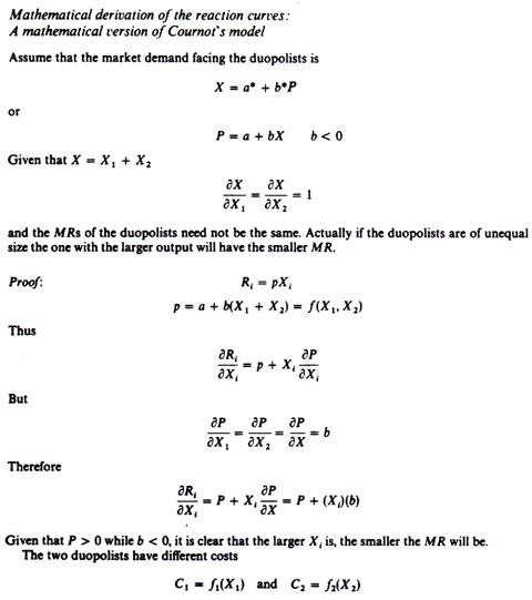
The first duopolist maximises his profit by assuming X₂ constant, irrespective of his own decisions, while the second duopolist maximises his profit by assuming that X₁ will remain constant.

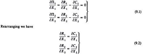
The first-order condition for maximum profits of each duopolist is

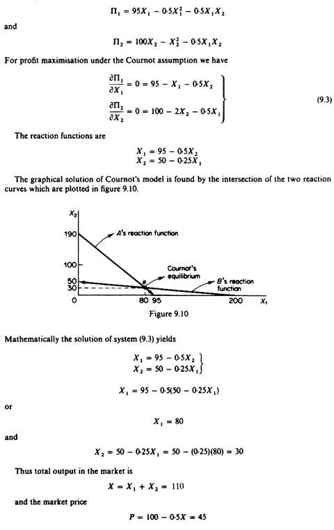
Solving the first equation of (9.2) for X₁ we obtain X₁ , as a function of X₂, that is, we obtain the reaction curve of firm A. It expresses the output which A must produce in order to maximise his profit for any given amount X₂ of his rival.

Solving the second equation of (9.2) for X₂ we obtain X₂ as a function of X₁, that is, we obtain the reaction function of firm B.

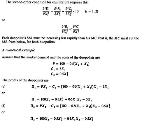
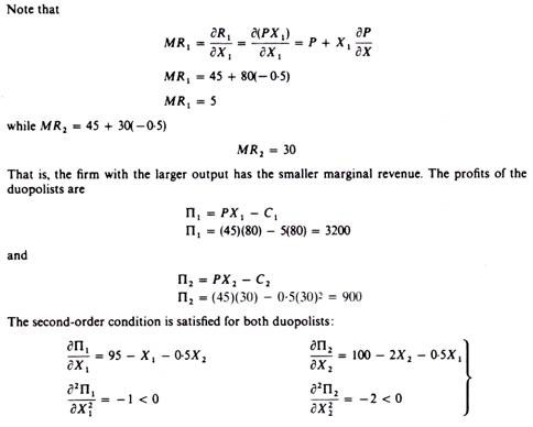
If we solve the two equations simultaneously we obtain the Cournot equilibrium, the values of X₁ and X₂ which satisfy both equations; this is the point of intersection of the two reaction curves.