Cases of Price Leadership (With Diagram)

Price leadership is said to exist when the price at which most or all of the firms in the industry offer to sell is determined by the leader (one of the firms of the industry).

This method was formulated by the German economist. Prof. Heinrichvon Stackelberg. This is also known as leadership solution or followership solution.

Here, we shall discuss three important cases of price leadership:

(1) Price Leadership by a Low-Cost Firm, and

(2) Price Leadership by a Dominant Firm.

(3) The Barometric Price Leadership Model

1. The Low-Cost Price Leadership Model:

In the low-cost price leadership model, an oligopolistic firm having lower costs than the other firms sets a lower price which the other firms have to follow. Thus the low-cost firm becomes the price leader.

Assumptions:

The low-cost firm model is based on the assumptions of:

1. There are two firms A and B.

2. Their costs differ. A is the low-cost firm and B is the high-cost firm.

3. They have identical demand and MR curves. The demand curve faced by them is 1/2 of the market demand curve.

4. The number of buyers is large.

5. The market industry demand curve for the product is known to both the firms.

Explanation:

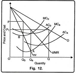
In Figure 12, D is the industry demand curve and d/MR is its corresponding marginal revenue curve which is the demand curve for both the firms and mr is their marginal revenue curve. The cost curves of the low-cost firm A are AC_a and MC_a and of the high-cost firm B are AC_b, and MC_b.

If the two firms act independently, the high cost firm B would charge OP price per unit and sell OQ_b quantity, as determined by point B where it’s MC_b, curve cuts the mr curve. Similarly, the low- cost firm A would charge OP₁ price per unit and sell OQ _a quantity, as determined by point A where its MC_a curve cuts the I curve. As there is a tacit agreement between the two firms, the high-cost fir leader firm A.

It will, therefore, sell OQ quantity, at a lower price OP₁ even though it will not be earning maximum profits. On the other hand, the price leader A will earn much higher profits at OP₁ price by selling OQ_a quantity.

Since both A and B sell the same quantity OQ_a the total market demand OQ is equally divided between the two, OQ = 2 OQ_a. But if firm B sticks to OP price, its sales will be zero because the product being homogeneous, all its customers will shift to firm A.

The price-leader firm A can, however, drive firm B out of the market by setting a lower price than OP₁, lower than the average cost AC_b, of firm B. Firm A would become a monopoly firm. But in such, a situation it will have to face legal problems. Therefore, it will be in its interest to fix OP₁ price and tolerate firm B in order to share the market equally and maximize its profits.

Price leadership model with unequal market Shares. The two firms will have different demand curves along with their different cost curves. The low-cost firm’s demand curve will be more elastic than that of the high-cost firm.

The high-cost firm would maximize its profits by selling less at a higher price while the low-cost firm would sell more at a lower price and maximize its profits. If they enter into a common price agreement, the high-cost firm will sell more quantity at a lower price set by the price leader by earning a little less than the maximum profits. But this is only possible so long as the price set by the leader covers the AC of the high-cost firm.

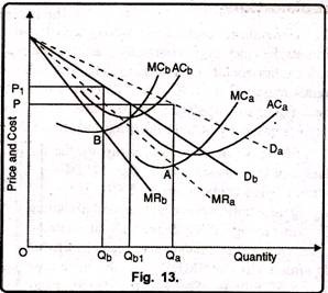
The price leadership model with unequal market shares is given in Figure 13, where the market demand curve is not shown to simplify the analysis. In the figure, D_a is the demand curve of the low-cost firm A and MR_a is its marginal revenue curve.

The demand curve and MR curve of the high-cost firm B are D_b, and MR_b, The low- cost firm A sets the price OP and the quantity OQ_a when its MC_a curve cuts its MR_a curve at point A. The price OP₁ and the quantity OQ/, of the high-cost firm B are determined when its MC_b, curve cuts its MR_b, curve at point B. Following the price leader firm A, when firm B accepts the price OP, it sells more quantity OQ_a1 and earns less than maximum profits.

It will pay the follower firm to sell this quantity at OP price so long as this price covers its average cost. If it does not follow the leader firm and tries to sell OQ₁, quantity at its profit maximisation price OP₁, it will have to close down because its customers will switch over to the leader firm which charges low price OP.

However, if there is no agreement for sharing the market between the leader and the follower firms, the follower can adopt the price of the leader (OP) but produce a lower quantity (less than OQ_b1) than required to maintain the price in the market, and thus push the leader to a non-profit maximisation position by producing less output.

2. The Dominant Firm Price Leadership Model:

This is a typical case of price leadership where there is one large dominant firm and a number of small firms in the industry. The dominant firm fixes the price for the entire industry and the small firms sell as much product as they like and the remaining market is filled by the dominant firm itself. It will, therefore, select that price which brings more profits to itself.

Assumptions:

This is based on the following assumptions:

1. The oligopolistic industry consists of a large dominant firm and a number of small firms.

2. The dominant firm sets the market price.

3. All other firms act like pure competitors, which act as price takers. Their demand curves are perfectly elastic for they sell the product at the dominant firm’s price.

4. The dominant firm alone is capable of estimating the market demand curve for the product.

5. The dominant firm is in a position to predict the supplies of other firms at price set by it.

Explanation:

Given these assumptions, when each firm sells its product at the price set by the dominant firm, its demand curve is perfectly elastic at that price. Thus its marginal revenue curve coincides with the horizontal demand curve.

The firm will produce that output at which its marginal cost equals marginal revenue. The MC curves of all the small firms combined laterally establish their aggregate supply curve. All these firms behave competitively while the dominant firm behaves passively. It fixes the price and allows the small firms to sell all they wish at that price.

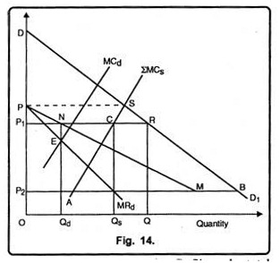
The case of price leadership by the dominant firm is explained in Fig. 14. DD₁ is the market demand curve. 2MC_S. is the aggregate supply curve of all the small firms.

By subtracting 2MC₅ from DD) at each price, we get the demand curve faced by the dominant firm, PNMBD₁ which can be drawn as follows:

Suppose the dominant firm sets the price OP. At this price, it allows the small firms to meet the entire market demand by supplying PS quantity. But the dominant firm would supply nothing at the price OP. Point P is, therefore, the starting point of its demand curve. Now take a price OP₁ less than OP.

The small firms would supply P₁ C (= OQ_s) output at this price OP₁ when their SMC_s curve cuts their horizontal demand curve P₁R at point C. Since the total quantity demanded at OP₁ price is P₁R (= OQ) and the small firms supply P₁C quantity, CR (= Q_s Q) quantity would be supplied by the dominant firm. By taking P₁N = CR on the horizontal line P₁R, the dominant firm’s supply becomes P₁N (= OQ_d). Thus we derive point N on the dominant firm’s demand curve by subtracting the horizontal distance from point P₁ to N from the demand curve DD₁.

Since the small firms supply nothing at prices below OP₂ because their ΣMC_s curve exceeds this price, the dominant firm’s demand curve coincides with the horizontal line P₂B over the range MB and then with the market demand curve over the segment BD₁. Thus the dominant firm’s demand curve is PNMBD₁.

The dominant firm will maximize its profits at that output where its marginal cost curve MC_d cuts its MR_d, the marginal revenue curve. It establishes the equilibrium point E at which the dominant firm sells OQ₁ output at OP₁ price.

The small firms will sell OQ_s output at this price for ΣMC_s, the marginal cost curve of the small firms equals the horizontal price line P₁R at C. The total output of the industry will be OQ = OQ_d + 0Q₅. If OP₂ price is set by the dominant firm, the small firms would sell P₂A and the dominant firm AB. In case a price below OP₂ is set the dominant firm would meet the entire industry demand and the sales of the small firms would be zero. The above analysis shows that the price- quantity solution is stable because the small firms behave passively as price-takers.

3. The Barometric Price Leadership Model:

The barometric price leadership is that in which there is no leader firm as such but one firm among the oligopolistic firms with the wisest management which announces a price change first which is followed by other firms in the industry. The barometric price leader may not be the dominant firm with the lowest cost or even the largest firm in the industry. It is a firm which acts like a barometer in forecasting changes in cost and demand conditions in the industry and economic conditions in the economy as a whole.

On the basis of a formal or informal tacit agreement, the other firms in the industry accept such a firm as the leader and follow it in making price changes for the product.

The barometric price leadership develops due to the following reasons:

1. As a reaction to the earlier experience of violent price changes and cut-throat competition among oligopolistic firms, they accept one firm as the price leader.

2. Most firms do not possess the expertise to calculate cost and demand conditions of the industry. So they leave their estimation to one leader firm which has the ability to do so.

3. Oligopolistic firms accept one among them as the barometric leader firm which possesses better knowledge and predictive power.