Study Notes on Isoquants ( With Diagram)

The below mentioned article provides an overview on isoquants which is a different combinations of two factors of production that are just physically able to produce a given quantity of a particular good.

Introduction:

We consider the production of a good, X, and suppose that only two factors of production— labour and capital—are employed.

Suppose also that it is always possible to substitute capital for labour and labour for capital continuously in the production process.

On the basis of these assumptions, it is possible that a given quantity of good X can be produced using different combinations of labour and capital. This is shown in Fig. 6.3, where the vertical axis measures units of capital (K) and the horizontal axis measures units of labour (L).

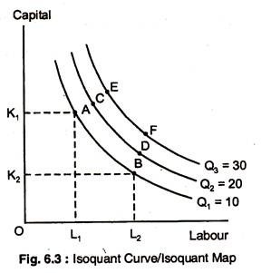
Point A represents just one possible combination of K and L which can be used to produce Q₁ units of output. There are, in fact, an infinite number of other points on the isoquant Q₁ all of which represent different combinations of K and L which can be used to produce Q₁ units.

Output Q₂ and Q₃ can be produced using any of the combinations of K and L represented by points along the isoquants.

An isoquant — or isoproduct — curve is a contour line which joins together the different combinations of two factors of production that are just physically able to produce a given quantity of a particular good.

For example, at A, 1 unit of labour and 3 units of capital yield Q₁ = 10 units of output, whereas, at D, the same output can be produced by 3 units of labour and 1 unit of capital. Similarly, Q₂ = 20 measures all combinations of inputs that yield 20 units of output. Q₂ produces more output than Q₁, and Q₃ > Q₂.

An isoquant map is a family of isoquants which shows the production function for a good.

The isoquants have three important properties:

(1) No two isoquants can intersect;

(2) Isoquants slope downwards from left to right;

(3) They are convex to the origin.

These properties are considered, in turn.

Isoquants cannot Intersect:

Isoquants, are similar to the indifference curves that we used to study consumer theory. Where indifference curves order levels of satisfaction from low to high, isoquants order levels of output. However, unlike IC_s, each isoquant is associated with a specific level of output.

By contrast, higher level of utility are associated with higher IC_s, but we cannot measure the specific level of utility the way we can measure a specific level of output with an isoquant.

An isoquant map is a set of isoquants, each of which shows the maximum output that can be achieved for any set of inputs. An isoquant map is an alternative way of describing a production function, just as an indifference map is a way of describing a utility function. Each isoquant is associated with a different level of output, and the level of output increases as we move up and to the right in the figure.

Fig. 6.4 shows two intersecting isoquants, Q₁ and Q₂. As drawn, point H represents a combination of K and L, which, when used efficiently, can apparently produce two different quantities of good X — Q₁ units and Q₂ units. This absurd result confirms the statement that isoquants cannot intersect.

Isoquants are Negatively Sloped:

If both capital and labour have positive marginal products, then it follows that to maintain a given level of output when the quantity of one factor is reduced, the quantity of the other must be increased.

Isoquants are Convex to the Origin:

If labour and capital are substitutes for each other, then isoquants must be convex to the origin. As bigger quantities of labour and smaller quantities of capital are employed to produce a given level of output, labour becomes less and less capable of substituting for capital.

Similarly, as bigger quantities of capital and smaller quantities of labour are employed to produce the same level of output, capital becomes less and less capable of substituting for labour. We can see in Fig. 6.5 that as the quantity of capital employed is reduced by one unit from OA to OB, the quantity of labour employed must increase from OD to OE for output to remain unchanged at Q₁.

If the quantity of capital is now reduced again by one unit to OC, the quantity of labour employed must increase to OF to maintain output at Q₁: Clearly, EF is bigger than DE. Thus, as more and more units of capital are given up, successively larger quantities of labour must be hired in order to keep the output level unchanged.

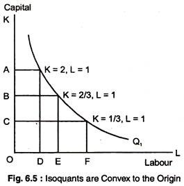
The slope of the isoquant measures the rate at which capital can substitute for labour, keeping output constant. This slope is called the marginal rate of technical substitution of capital for labour (MRTS). Isoquants are downward-sloping and convex like indifference curves. On isoquant Q₁, the MRTS falls from 2 to 1 to 2/3 to 1/3. Isoquants are convex — the MRTS diminishes as we move down along an isoquant.

The diminishing MRTS tells us that the productivity that any one input can have is limited. As a lot of labour is added to the production process in place of capital, the productivity of labour falls. Similarly, when a lot of capital is added in place of labour, the productivity of capital falls.

Production needs a balanced mix of both inputs. The MRTS is closely related to the MP_L and MP_K We can see that adding some labour and reducing some capital keep output constant.

Additional output from increased use of labour – MP_L x ΔL

Similarly, reduction of output from decreased use of capital = MP_K x ΔK. Since we are keeping output constant by moving along an isoquant, the total change in output must be zero. Thus,

MP_L x ΔL + MP_k x ΔK = 0

.^.. MP_L/MP_K = – ΔK/ΔL = MRTS.

Production with Two Variable Inputs:

Now that we have seen the production relationship, let us reconsider the firm’s production technology in the long-run, where both capital (K) and labour (L) inputs are variable. We can examine the alternative ways of producing by looking at the slope of a series of isoquants.

As we know, an isoquant describes all combinations of inputs that yield the same level of output. The isoquants slope downward because both labour and capital have positive marginal products. More of either input increases output; so if output is to be kept constant as more of one input is used, less of other input must be used.

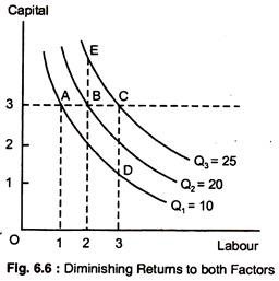
Diminishing Returns:

There are diminishing return to both inputs. To see why there are diminishing returns to labour we draw a horizontal line at a particular level of capital, say 3 units. Reading the levels of output from each isoquant as labour is increased, we note that each additional unit of labour generates less and less output. For example, when labour is increased from 1 unit to 2 (from A to B), output increases by 10.

However, when labour is increased by an additional unit (from B to C), output increases by only 5. Thus, there are diminishing returns to labour—both in the long and short-run. While adding one factor keeping, the other factor constant eventually leads to lower level of output, the isoquant must become steeper, as more capital is added in place of labour, and flatter when labour is added in place of capital.

There are also diminishing returns to capital. With labour fixed, the marginal product of capital decreases as capital is increased. For example, when capital is increased from 1 to 2 units and labour is held constant at 3, the marginal product of capital is initially 10, but the marginal product falls to 5 when capital in increased from 2 to 3, as Fig. 6.6 shows.

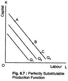
Production Function when Inputs are perfectly substitutable:

When the production isoquants are straight lines, the MRTS is constant. This means that the rate at which capital and labour can be substituted for each other is the same whatever level of inputs is being used, as Fig. 6.7.

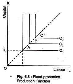
Fixed-proportion Production Function:

When the production isoquants are L-shaped, only one combination of labour (L) and capital (K) can be used to produce a given output. The addition of more labour does not increase output, nor does the addition of more capital alone, which has been shown in Fig. 6.8.

Isocost Lines:

An isocost line shows all the combinations of capital and labour that can be bought for a given monetary outlay. If we draw the isocost and the isoquant map together, this will enable us to identify the cost-minimising combination of factors that a profit-maximising firm will employ to produce its chosen output level.

Suppose that the price of labour is £2 per unit and the price of capital is £1 per unit. Table 6.4 shows the combination of the two factors that can be bought for an outlay £20. These combinations are plotted as the isocost line AB in Fig. 6.9.

The slope of the line (OA/OB = 2) represents the relative factor price ratio. The isocost line for an outlay of £40 is plotted A ‘B’ on the graph and it is parallel to AB. Similarly, the isocost line for a £10 outlay, A “B” is also parallel to AB.

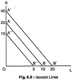
A change in the relative factor price ratio will change the slope of the isocost lines.