When is Price Discrimination Profitable? | Monopoly

We shall now derive the condition for profitability of price discrimination. For the sake of simplicity we shall assume that the firm is a single-plant monopolist, and it is selling its product in only two markets. Also, let us suppose that the firm finds that price discrimination between the two markets is possible and it has decided to discriminate if it is profitable. By definition, at any output (q) we have,

profit of the firm (π) = total revenue (TR) – total cost (TC)                                (11.33)

The firm’s TR and TC are functions of q (quantity of output produced and sold), and so its n also is a function of q. That is why, at different values of q, we would have to know the values of TR and TC, and of n, and, in the process, we would be able ultimately to have the firm’s maximum π and the q at which that n is obtained.

Now, at different qs, the firm’s (minimum required) TCs are obtained from its TC function. It may be noted here that since the firm is a single-plant monopolist, the determination of the (minimum) cost of producing a particular quantity of output does not require any consideration of how the production of the output is distributed between the different plants.

On the other hand, the firm’s TRs at different qs are obtained from its TR function. But here, since the firm is selling in two different and separated markets, determination of maximum TR at any particular q depends upon how the sale of the output (q) is distributed in the two markets. The conditions for maximising TR, i.e., for maximising n (TC being given), at any particular q, may be obtained in the following way.

In this two-market case the TR at any q is

TR=TR₁(q₁) + TR₂(q₂)

= TR(q₁, q₂) (11.34)

subject to q₁ + q₂ = q = constant.

Here, q₁ and q₂ are the quantities of output respectively sold in the two markets, and TR₁ and TR₂ are the respective TRs in the two markets.

Now the first order or necessary conditions (FOCs) for maximum TR are

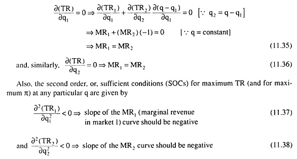
Since it follows from the features of monopoly that MR function in each market would be negatively sloped, the SOCs given above already stand satisfied. Now, the FOC, i.e., MR₁ = MR₂ gives us that any particular quantity of output, q, should be sold in the two markets in such quantities, i.e., the values of q₁ and q₂, (q₁ + q₂ = q), should be such that the marginal revenues in the two markets may become the same.

For, if the q is distributed between the two markets in a manner that makes MR₁ and MR₂ unequal, then the firm would be able to increase its TR, and, therefore, π (TC being given), by decreasing the output sold in the lower-MR market and increasing that in the higher-MR market.

Now, as the firm does this, the MR in the lower-MR market would be rising and the MR in the higher-MR market would be falling, since the MR functions are negatively sloped, and at some distribution, in the process, the two MRs would become equal to each other.

It would no longer be possible for the firm to increase its TR and n at the q under consideration, by shifting the marginal units from one market to another. Therefore, at this distribution, with MR₁ = MR₂, the firm’s TR and n would be maxi­mum for the particular q.

We have seen, therefore, that distribution of the sale of each particular q between the two markets, according to the MR₁ = MR₂ rule, would ensure that the firm earns maximum profit from selling any particular quantity of output.

Now, the maximum of these maximum profits for different qs is what the firm would want to earn at the equilibrium point. That is, here the firm’s aim is to earn the maximum maximorum of profit.

For the time being let us note that if the discrimi­nating monopolist is to achieve his ultimate goal of profit maximisation, then in order to derive his TR function, he would have to distribute each quantity of sale between the two markets in a way so that the MR₁ = MR₂ rule is satisfied.

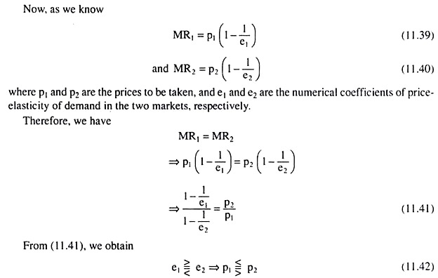
Eqn. (11.42) gives us that the MR₁ = MR₂ rule or profit maximisation requires the prices to be different in the two markets only when elasticities of demand there are different—the price in the higher-elasticity market would be smaller than the price in the lower-elasticity market.

In other words, price discrimination would be profitable only when the elasticities in different markets are different. (11.42) also gives us that if the elasticities in the two markets are equal, i.e., if the markets are iso-elastic, then price-discrimination is not profitable. In the case of iso-elasticity, profit maximisation requires the prices to be the same (p₁ = p₂) in the different markets.

Equilibrium of a Price-Discriminating Monopolist:

We are assuming here that:

(i) Price discrimination is possible and profitable,

(ii) The monopo­listic firm wants to achieve profit maximisation by means of price discrimination, and

(iii) The firm has decided to discriminate between the two geographically separated markets with re­spect to price.

We have to derive the conditions for profit-maximising equilibrium of the firm.

We have seen that at any particular quantity of output (q) produced and sold, the price-discriminating firm would be able to maximise its total revenue (TR) and profit (n) if it distributes the sale of the output between the two markets in a way such that the MRs in both the markets become the same (MR₁ = MR₂).

It may be noted here that MR₁ = MR₂ itself is the MR at any particular q, i.e., we may write MR₁ = MR₂ = MR. We may understand the point with the help of a simple example. Let us suppose that at any particular q = 1,000 units, if the firm sells q, = 600 units in the first market and q₂ = 400 units in the second market, then we have MR₁ = MR₂ = Rs 50.

In this case, the marginal unit of q₁ i.e., the 1,000th unit, is either the 600th unit of q₁ or the 400th unit of q₂. In whatever market this marginal unit (i.e., the 1,000th unit) is sold, the incre­ment in the TR of the firm would be Rs 50, i.e., the MR at q = 1,000 units would be MR₁ = MR₂ = MR = Rs 50.

Let us also note here that if the MR₁ and MR₂ functions are negatively sloped as they would be under monopoly, then the firm’s MR function also would be negatively sloped. Because, as q increases, sales in both the markets would increase and MR₁ = MR₂, i.e., MR of the firm would fall.

Now, if at any q₁ the firm has MR₁ = MR₂ = MR > MC (marginal cost), then it would have a positive profit from the production and sell of the marginal unit (MR – MC > 0), and, in that case, the profit-maximising firm would have to increase its q.

For, marginal profit being posi­tive, the firm’s total profit would rise as q increases. On the other hand, if at any q, the firm has MR₁ = MR₂ < MC, then the firm would have a negative profit on the margin and, in that case, the profit maximising firm would have to reduce its q.

For, the marginal profit being negative, the firm’s total profit will rise as q decreases. However, if at any q₁ the firm has MR₁ = MR₂ = MC, its marginal profit will be zero, and it would have no reason either to increase or to decrease its q, for, by going either way, it can no longer increase, rather would decrease, its profit.

That is why q = q* would be the firm’s equilibrium or profit-maximising output and the condition for achieving this equilibrium is

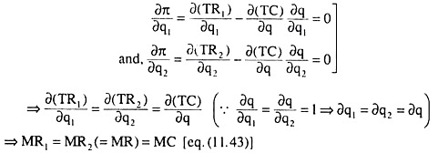
MR = MR₁ = MR₂ = MC                               (11.43)

(11.43) is the first order or the necessary condition (FOC) for the profit-maximising equilibrium of the firm. For we have seen, so long as MR, = MR₂ ≠ MC, the firm cannot be in equilibrium and for the firm to be in equilibrium, it is necessary that condition (11.43) is satisfied.

But condition (11.43) is not the sufficient condition for profit maximisation, because satis­faction of this condition does not guarantee profit maximisation.

For example, if at q = q*, i.e., at the point where (11.43) is satisfied, the MR curve after intersecting the MC curve goes above the latter, then the firm would not be in equilibrium at q = q*—rather, it would increase its output, for, by doing that, it would be able to increase its level of profit.

Therefore, the second order or sufficient condition (SOC) for profit maximisation is that, at q = q*, the MC curve after intersecting the MR curve must go above it. For then, if the firm proceeds beyond q = q*, its profit level would decline, MC becoming greater than MR.

We may now illustrate the equilibrium of the discriminating monopolist with the help of Fig. 11.21. In Fig. 11.21(a), the AR, and MR, curves are the average and marginal revenue curves of the firm in the first market, and in Fig. 11.21(b), the AR₂ and MR₂ curves are those curves in the second market. For the sake of simplicity, the AR and MR curves in the two markets have been drawn as straight lines.

In Fig. 11.21, we have, by construction, e₁ < e₂, for the AR, curve is steeper than the AR₂ curve and the vertical intercept of the AR, line is greater than that of the AR₂ line. In Fig. 11.21(c), the MR (= MR₁ = MR₂) curve is the horizontal summation of the MR, and MR₂ curves. We obtain from this line what would be the MR, = MR₂ (= MR) at any particular q sold. For example, at the output q* = oq*, the MR₁ = MR₂ (= MR) is q*E or OC.

How the quantity, q* = Oq*, is to be divided between the two markets so that we may get MR, = MR₂ = OC, can be obtained from Fig. 11.21(a) and 11.21(b) which shows us that if the firm sells q* = Oq* units of the output in market 1 and q*₂ = Oq₂ units of the output in market 2, then the MRs in both the markets would be the same, being equal to OC which would also be the MR of the total output (here q*).

By construction, we have q₁* + q*₂ =q*. In Fig. 11.21(c) the MC curve is the firm’s marginal cost curve, which gives us the firm’s MC at any particular quantity of output.

After we come to know which curve gives us what in Fig. 11.21, it has now become easy for us to pick up the equilibrium point of the firm. In Fig. 11.21(c), the point of intersection, E, between the curves MR (= MR₁ = MR₂) and MC, is itself the equilibrium point of the firm.

For at the point E or at the firm’s output of q* = Oq*, the FOC (11.43) and also the SOC of firm’s equilibrium have been satisfied. For, at the point E, we have MR = MR₁ = MR₂ = MC, and also the MC curve is upward sloping.

Lastly, we find in Figs. 11.21(a) and 11.21(b) that, of the equilibrium output q*, q* would be sold in the first market at the price p₁ = p* and q*₂ would be sold in the second market at the price p₂ = p*₂. We also have p*₁ > p*₂, i.e., the price in the less elastic market (here market 1) would be more than that in the more elastic market (here market 2) [Eqn. (11.42)].

We may now derive the conditions for the discriminating firm’s profit-maximising equilibrium with the help of calculus. For such a firm we obtain

Now, calculus gives us the FOCs for maximum π as

Let us now come to the SOCs for maximum π that are given by the principal minors of the determinants D given below alternating in sign starting from the negative;

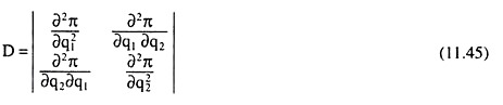
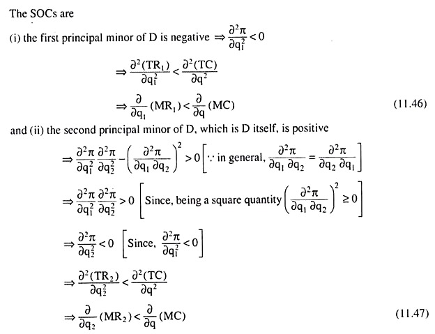
The SOCs (11.46) and (11.47) give us that, at the point where the FOC (11.43) is satisfied, i.e., at the point of intersection (E) between the MR (= MR₁ = MR₂) and the MC curves in Fig. 11.21(c), i.e., at q*₁ = Oq*₁ and q*₂ = Oq*₂ in Figs. 11.21 (a, b), the rate of change of MR₁ w.r.t. q₁ and the rate of change of MR₂ w.r.t. q₂ should be less than the rate of change of MC w.r.t. q.

Price Discrimination between a Monopolistic Market and a Competitive Market:

Sometimes a monopolistic firm may have to sell its product in the home market as also in the competitive foreign market, i.e., in the home market, the firm is a monopolist, but in the foreign market, it is a perfect competitor. In this case, elasticity of demand (e), is different in the two markets. In the home market, e is finite and in the foreign market, e is infinitely large (e = ∞).

Therefore, price discrimination between the two markets is profitable—the firm would have to charge a higher price in the home market and a lower price in the foreign market. Also, price discrimination is possible in this case, the two markets being geographi­cally separated. We shall explain the profit-maximising equilibrium of such a discriminating monopolist with the help of Fig. 11.22.

In Fig. 11.22, the curves AR_m and MR_m (drawn as straight lines for the sake of simplicity) are the average and marginal revenue (AR and MR) curves, respectively, of the firm’s monopo­listic home market. As regards the perfectly competitive foreign market, let us suppose that the price of the product in this market is p_c = Op_c.

The firm is a price-taker in this market. At this price, it can sell, more or less, any quantity of its product. Therefore, its AR = MR curve in this market will be a horizontal straight line AR_C = MR_C at the level of Op_c.

The monopolistic firm’s MR = MR_C = MR_m curve, or the combined MR curve as it may be called, would be obtained as the curve ABED in Fig. 11.22—this curve, would be the hori­zontal summation of the MR_C and MR_m curves.

There­fore, the point of intersection, E, of the ABED and MC curves would be the equilibrium point of the monopolist. For, along with the FOC (i.e., MR_C = MR_m = MR), the SOC also has been satisfied at E, since the MC curve is upward sloping while the (com­bined) MR curve is horizontal at this point. There­fore, the equilibrium output of the firm would be q* = Oq*.

Of this quantity the firm would sell q_m = Oq_m units at the price p_m = Op_m in the monopolistic (home) market, and it would sell the rest of the output, i.e., Oq* – Oq_m, in the competitive foreign market where the price is given to be p_c = Op_c.

It may be noted that since e is smaller in the monopolistic market than in the competitive market, the firm would charge a higher price (p_m) in the former market and a lower price (p_c) in the latter market (p_m > p_c).

Block Pricing and Perfect Price Discrimination:

Price discrimination occurs, when a monopolist charges his customers different prices of his product at the same time. Here we shall discuss a form of price discrimination when a monopolist sets different prices for the same consumer or for the same market.

This type of price discrimination is also known as volume discounts or block pricing. For exam­ple, the monopolist may charge the consumer a higher unit price for the first 10 units of the good than for the next 10 units.

In order to explain this phenomenon, we have to remember the principles of the Marshallian analysis of consumer behaviour (single commodity case), Let us also suppose that a particular consumer’s demand curve for the good (which is also his marginal utility curve) is given by AB in Fig. 11.23.

It is seen from this curve that at any price p₀, the consumer is willing to buy the quantity, q₀, of the good. In this case, let us remember, his marginal utility (MU) is p₀, and he would earn a total utility (TU) equal to area OACq₀ and is spending a total amount of money equal to area Op₀Cq₀, i.e., the monopolist’s total revenue from selling q₀ units of output at p = p₀ would be

TR₁ = □Op₀Cq₀.

Therefore, in this case, consumer would have a net surplus of utility, called consumer’s surplus, equal to □OACq₀ – □Op₀Cq₀ = □Ap₀C. Now, if the monopolist knows the consumer’s demand curve as given in Fig. 11.23, then he finds that when he charges a higher price, say, p₁ (> p₀), the consumer would demand the quantity q₁ (< q₀).

He also finds that if, in this case, he charges the consumer the price, p₁, for the first q, units and the price, p₀, for the next (q₀ – q₁) units, then he would be able to increase his total revenue of selling the same q₀ units to the consumer over and above TR₁. For, now, his total revenue or the consumer’s total expenditure would be

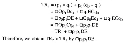
That is, if the monopolist resorts to block pricing, then his TR, or, the consumer’s total expenditure at any particular quantity of output (here q = q₀), would rise and so his profit (= TR -TC) would rise, and the consumer’s surplus (= TU-total expenditure) would fall (here by the area p₀p, DE). This is because the monopolist’s total cost of producing the said quantity and the consumer’s total utility derived remain the same.

Similarly, if the monopolist charges p = p₂ for the first q₂ units of his output of q₀, p = p₁ for the next q₁ – q₂ units and p = p₀ for the next q₀ – q₁ units of his output, then he would be able to increase his TR and also his profits or reduce the consumer’s surplus by a further amount = □p₁p₂FG.

We have explained above how block pricing helps to increase the monopolist’s TR and profit at any particular quantity of output by enabling him to appropriate a larger share of consumer’s surplus. Let us now come to perfect price discrimination.

In block pricing, if the number of blocks in which the monopolist divides any particular quantity of his output becomes larger, i.e., the size of the blocks becomes smaller, each block having a separate price, then, in the limit, each unit of the said quantity of output would constitute a separate block having its own price, i.e., each unit of the output would be sold at a different price, the price the consumer is willing to pay for the said unit.

For example, it is known from the consumer’s demand curve in Fig. 11.23, that he is willing to pay p = p₂ for the q₂th unit of output, p = p₁ for the q₁th unit of output, or p = p₀ for the q₀th unit of output, and so on.

Now, if the monopolist charges p = p₂ for the q₂th unit, p = p₁ for the q₁h unit, or p = p₀ for the q₀th unit, and so on, then it is obvious that for any unit, the price the consumer is willing to pay is equal to the price that he is required to pay, i.e., the utility that he is deriving from any unit becomes equal to the price that he would have to pay, leaving no surplus whatsoever for the consumer.

This phenomenon is known as perfect price discrimination. Here the monopolist would be able to appropriate 100 per cent of con­sumer’s surplus for himself thereby increasing his TR to the entire area under the consumer’s demand curve.

For example, in Fig. 11.23, if the consumer buys the quantity q = q₀ of the good, paying p = p₂ for the q₂th unit, p = p₁ for the q₁th unit, and so on, i.e., paying a different price for each unit, then the TR of the monopolist would be equal to EMU = TU that the consumer derives from consumption of this quantity, and consequently, his consumer’s surplus would be equal to zero. Both TR and TU here would be equal to □OACq₀.

Therefore, that in the case of perfect price discrimination, the TR obtained by the monopolist by selling any particular quantity would be the summation of all the different unit prices, i.e., TR would be equal to the area under the demand curve for that quantity. Also total utility (TU) obtained by the consumer is equal to the same area. Since TR = TU, here consumer’s surplus (= TU – TR) would be reduced to zero.

We have analysed above the phenomena of block pricing and perfect price discrimination. Let us note, however, that it is difficult for the monopolist to practice both these types of price discrimination because they require him to know beforehand the demand curve of a consumer which is a difficult job.

Even if this were possible, it would be prohibitively complicated to establish a different price policy for each and every individual consumer.

Nonetheless, some general schemes of block pricing and volume discounts applicable to all the consumers are often used by public utilities and telephone companies. These price police are explained in part by the presence of lumpy costs associated with providing service to individual consumers, but there is good reason to suspect that some sort of price discrimination also takes place.

Equilibrium under Perfect Price Discrimination:

In the case of perfect price discrimination, by definition, the monopolist charges the consumer for any unit of his product, a price which is exactly equal to the amount that the consumer is willing to pay.

That is why the consumer’s surplus is reduced to zero, and that is why the consumer’s demand curve which is the same as the monopolist’s demand curve (since the con­sumer himself constitutes the market for the monopolist’s product) becomes also the monopolist’s marginal rev­enue (MR) curve.

For example, if we observe in Fig. 11.24, that the consumer wants to pay the price p_n, p_n+1, p_{n + 2},…, for the q_nth unit, q_{n + 1}th unit, q_{n+ 2}th unit,. . ., of the good along his demand curve and the monopolist exactly charges these prices for said units of the good, then what is implied here is that for the q_nth unit, q_{n+ 1}th unit, q_n+2th unit, etc. the monopolist’s additional or mar­ginal revenues are respectively p_n, p_{n + 1}, p_{n + 2}, etc.

This gives us that the consumer’s or the monopolist’s demand curve DD may itself be treated as his MR curve.

Now, if the monopolist’s marginal cost curve is given to be MC in Fig. 11.24, then his equilibrium will occur at the point E which is the point of intersection of his MR and MC curves and which satisfies, therefore, the FOC for maximum profit.

At the point E, the SOC is also satisfied, since here the (negative) slope of the MR curve is less than the (positive) slope of the MC curve. At the point E, the monopolist produces and sells the output quantity q₀. How­ever, he does not sell all this output at the price p₀. Here p₀ is the price he takes for the q₀th unit or the marginal unit of output.

So p₀ may be called the marginal price. For all other units of output, he charges, as we know, what the consumer is willing to pay along his demand curve or the monopolist’s MR curve. For example, for the q_{n+ 1}th unit of output he charges the price p_{n + 1} and for the q_nth unit of output he charges the price p_n.

The monopolist maximises the amount of his profit at the point E or at the output of q₀ in Fig. 11.24. For, if q < q₀, he would find MR > MC, and hence, he would be willing to increase q. On the other hand, if q > q₀, he would find MR < MC, and hence, he would have to decrease q. He would increase or decrease q till MR becomes equal to MC at the point E, or, at q = q₀.

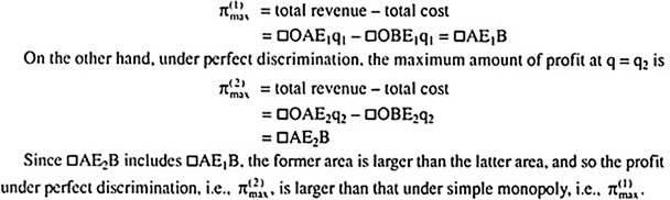
At q = q₀, the total revenue of the monopolist would be □OAEq₀ which is the area under the MR curve and his total cost would be □OBEq₀ which is the area under the MC curve. Therefore, the (maximum) amount of profit at q = q₀ would be DOAEq₀ – □OBEq₀ = □AEB.

It may be noted that the monopolist’s profit here includes the whole of consumer’s surplus = □AP₀E that the consumer might have obtained if all the units of output, q = q₀, were sold at the uniform price p = p₀.

Comparison between Simple Monopoly and Monopoly under Perfect Price Dis­crimination:

We may now easily compare the price-output equilibrium at maximum profit in simple mo­nopoly with that in monopoly under perfect price discrimination. In Fig. 11.25, DD is the demand curve of a consumer for the monopolist’s product. The consumer constitutes the market for the product. So DD is also the simple monopolist’s demand or average rev­enue (AR) curve.

The corresponding marginal revenue curve is MR. If the marginal cost curve is MC, then the simple monopolist’s equilibrium point is the MR – MC intersection point E₁. At E₁, the FOC for maximum profit, i.e., MR = MC, has been satisfied as also the SOC, for here the slope (negative) of the MR curve is less than the slope (positive) of the MC curve. At E₁, the simple monopolist’s equilib­rium output quantity is q₁.

Let us now come to the case of the monopolist under perfect price discrimination. Here the DD curve itself is his MR curve and his MR = MC point is E₂ where the FOC for maximum profit has been satisfied as also the SOC, for here the slope (negative) of the MR (which is DD here) curve is less than the slope (positive) of the MC curve.

At E₂, the equilibrium output quantity under perfect price discrimination is q₂. Since the points E₁ and E₂ both lie on the upward sloping MC curve and E₂ lies upward towards right of E₁, the equilibrium output under perfect price discrimination is greater than that of the sim­ple monopolist, i.e., q₂ > q₁.

Let us now come to the equilibrium price of the product in the two situations. The uniform profit-maximising price of the simple monopolist at q = q₁, is p = p₁ which is obtained at the point F, on the DD curve. On the other hand, under perfect price discrimi­nation each unit of output is charged a different price.

Here the marginal price, i.e., the price charged for the marginal unit of equilibrium output, q₂, is p₂ which is obtained at the point E₂ on the DD curve.

Since E₂ lies downward towards right of F₁, we have p₂ < p₁, i.e., the marginal price under perfect discrimination is smaller than the uniform price under simple monopoly.

Also, for any output larger than q, and smaller than or equal to q₂, we obtain the marginal price under perfect discrimination to be less than the uniform price of the simple monopolist, and for any output smaller than or equal to q₂, we obtain the mar­ginal price under perfect discrimination to be greater than or equal to the uniform price under simple monopoly.

Lastly, let us compare the maximum amounts of profit that are obtained in the two situa­tions. Under simple monopoly, the maximum amount of profit at q = q₁, is

 

 

 

 

 

 

 

Is Price Discrimination Desirable?

We may examine whether price-discrimination is desirable from the point of view of the buyers and sellers of the product concerned and also from the point of view of society. Price-discrimi­nation is advantageous to those buyers who can purchase the product at a lower price.

Gener­ally, the buyers with a smaller purchasing power would have a higher price-elasticity of de­mand and they would be asked to pay a lower price, and the buyers with a larger purchasing power would have a lower price-elasticity of demand, and they would be asked to pay a higher price. Therefore, price-discrimination is also socially desirable.

Although price-discrimination helps the monopolist to earn a larger amount of profit, and therefore, may not be deemed desirable, the argument has another side also. A losing monopo­listic concern, by charging its richer customers a higher price and the poorer customers a lower price, may be able to earn at least the normal profit.

In this case, price discrimination is very much desirable. For, if the firm did not discriminate, it would have closed down, and conse­quently, the consumers would have suffered and the employment and output of the society would have reduced.

However, in most cases, the monopolistic firms are not losing concerns, they are driven by profit motive and if price discrimination is possible and profitable, they will discriminate to earn more profit—they will charge a higher price in some market but not set a sufficiently lower price in another market. Therefore, on balance, price discrimination may not be desirable.