Monopoly Market: 5 Things to Know about Monopoly Market

Monopoly Market # 1. Meaning of Monopoly: 

‘Mono’ means one and ‘poly’ means seller. Thus, monopoly refers to a market situation in which there is only one seller of a particular product.

Here the firm itself is the industry and the firm’s product has no close substitute. The monopolist is not bothered about the reaction of rival firms since it has none. The demand curve of the monopolist is the industry demand curve. (Recall that in pure competition there are two demand curves).

Can there be complete monopoly in the real commercial world? Some economists feel by maintaining some barriers to entry a firm can act as the single seller of a product in a parti­cular industry. Others feel that all products compete for the limited budget of the consumers. Therefore, no firm, even if it is the only seller of a particular product, is free from competition from the sellers of other products. Thus, complete monopoly does not exist in reality.

Monopoly Market # 2. Profit-Maximising Output under Monopoly:

We have developed two rules of profit- maximisation. The first rule —the shut-down rule—applies straightaway to monopoly. But the second rule—i.e., the MR-MC rule—has to be slightly modified in case of monopoly because MR is not equal to P.

Marginal Revenue of a Monopolist:

Since a firm under perfect competition can sell as much as it likes at a growing price, its MR = P. By contrast, a monopolist, being the sole supplier of a commodity, cannot do so. It is because the demand (average revenue) curve faced by monopolist is the same as the market demand curve of the industry.

The market demand curve is always downward sloping. The implication is that the mono­polist has to reduce the price to sell one extra unit. Since it has to reduce the price of all the units sold (and not just the price of the last unit) the marginal (extent) revenue obtained by selling one extra unit is less than the price at which all units are sold.

Let us consider a simple example: 

Suppose a monopolist is selling 3 units of a commodity per day at a price of Rs. 60. His total revenue is Rs. 180. Now, suppose he wants to sell the fourth unit. This is possible if he reduces the price to Rs. 50. Then, his total revenue will be Rs. 50 x 4 = Rs. 200. Thus marginal revenue is Rs. 200 – Rs. 180 = Rs. 20. This is less than the new price that he charges for his product, viz., Rs. 50.

In fact, MR is less than P for two reasons. Firstly, when the monopolist sells one extra unit (the fourth unit is an example) his total revenue increases by Rs. 50 (which is the price of the last unit). Secondly, there is a fall in TR due to the low price now charged on the first 3 units (i.e., Rs. 50 instead of Rs. 60 each). The fall in TR is, therefore, (Rs. 60 – Rs. 50) x 3 = Rs. 30.

Thus, MR can be calculated as follows:

Increase in TR from 1 unit at Rs. 50 = Rs. 50

Fall in TR from 3 units at Rs. 10 less = – Rs. 30

Net change in TR = Rs. 20

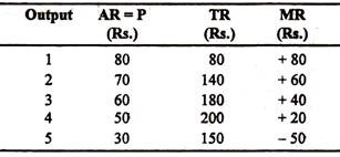
The following table gives the hypothetical revenue schedule of a monopolist:

It shows MR and AR at five different prices, at which it sells different quantities of its product. It is clear that the monopolist has to reduce the price to sell more. As a result MR and AR both fall.

But MR falls faster than AR. Therefore, both the MR and AR curves, when plotted, will be downward sloping but the MR curve will lie below the AR curve. Thus the important point to note is that MR is always less than AR whenever the demand curve is downward sloping.

Table 11.1: The revenue schedule of a monopolist

The gap between the two curves measures the degree of monopoly. From Table 11.1 we see that MR is always less than AR (=P), except for the first unit, when TR is the same as the increase in revenue between zero output and one unit of output.

By contrast the monopolist is the sole seller of a particular product. Therefore, if the monopolist is to enjoy excess profit in the long-run it must erect certain barriers to entry. Such barriers any refer to any force which prevents rival firms (competing producers) from entering the industry.

Such barriers which protect the monopolist from the encroachment of other firms may be either natural or man-made. Such type of barrier can take different forms. We may now make a brief review of some of the important barriers.

(a) Natural Barriers:

There are three sources of natural barriers.

These are the following:

(i) Cost advantage:

If production in an industry is subject to increasing return to scale or decreasing cost, long-run average cost will tend to fall with an increase in the size of the firm. Thus an increase in the size of the firm is desirable. In this context we may refer to the concept of natural monopoly. Natural monopoly exists when there is scope to product at minimum efficient scale.

As R.G. Lipsey and C. Harbury have rightly co­mmented:

“In such an industry, competition among firms will lead to the emergence of one large firm serving the whole market— since the largest firm always has lower costs, and hence can undersell any small competitions.”

(ii) Sole Control over a basic material:

A prime cause of cost advantage seems to be the possession of a critical raw material. This is another natural barrier to entry. For example, a cement manufacturing company may have sole access to a basic raw material, viz., limestone and may thus enjoy monopoly position in the industry. Similarly company may own a small piece of land beneath which oil is found.

(iii) Locational advantages:

Some locations offer special advantages than others. This fact discriminates in favour of certain firms and against others. This, in its turn, makes it im­possible on the part of potential new entrants to compete on equal terms with an estab­lished firm.

For example, a restaurant adjacent to a bus junction can expect more sales than those situated in remote places. A book shop in Dariaganj area of Delhi can expect more sales than another shop situated near the Delhi airport. Such locational advantages also give rise to cost advantages.

For example: 

Hindustan Lever’s soap factory near the Kidder-pore area of Calcutta is situated on the bank of river Hooghly. This proximity to a river lowers HL’s costs of waste disposal, compared to other firms.

(b) Artificial Barriers:

Artificial barriers are those which are created by human beings and not by nature. Some of these are created by individuals and business firms, while others are created by governments.

Such barriers are of the following broad categories:

(i) Product Differentiation:

This is an important feature of monopoly because it implies absence of close substitutes. Product differentiation enables a firm to deter the entry of new firms in the industry. This is often achieved through advertising and sales promotion. For example the Reckitt and Colman of India Ltd. is enjoying a virtual monopoly position as far as its main product, viz., Dettol is concerned. In spite of introduction of Savlon by ICI Ltd., Dettol continues to be the most popular antiseptic germicidal in the country.

(ii) Legal Barriers:

By using patents on production processes (as in the case of Coca Cola) and copyrights on publications (as in the case of Lipsey’s Positive economics by London’s George Weidenfeld and Nicolson Ltd.) legal restrictions may be imposed on the entry of new firms in an industry. Such legal devices are often used for preventing the entry of new firms in an industry.

(iii) Barriers Created by Government:

The Government can also create monopoly by giving the legal right to a company to produce a particular product or render a particular service. For example, the Acts of Parliament protect India’s nationalised industries such as the Coal India Ltd. or the LIC, at least partly, from competition of private firms. The State Governments also grant monopoly rights to private firms such as Roy’s Wine Shop in Salt Lake area of Calcutta, the only duty free shop in an airport, or the only service station in particular locality.

One may also note that MR is negative when the monopolist increases his sales from 4 to 5 units. Here it is clear that TR at a higher output (5 units) and lower price (Rs. 30 per unit) is less than TR at the lower output (4 units) and higher price (Rs. 50).

This is so because of the inelasticity of demand for the product. Here the numerical value of e_p is less than one. By contrast, in pure competition, MR is always equal to price, because e → ∞. Since price can never be zero (so as to make the commodity under consideration a free good like air or water) MR is always positive.

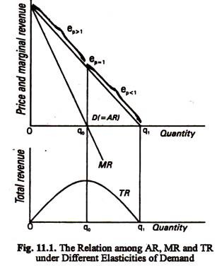
Thus, in monopoly, MR is negative as TR falls beyond a particular level of sales. This is due to inelasticity of demand. It is also poss­ible to show that if demand for the product of the monopolist is unitary elastic, price change will have no effect on TR and MR will be zero. (This is not possible in perfect competition). Thus it logically follows that the monopolist should never operate or the inelastic portion of its demand curve. This point is illustrated in Fig. 11.1.

Marginal Revenue and Price Elasti­city of Demand:

The relationship among TR, MR and AR is shown in Fig. 11.1. We know that elasticity of demand varies continuously along a straight line demand curve.

From Fig. 11.1, we discover two important features of the MR curve of a monopolist:

(a) The MR curve always lies below the AR curve (except for the first unit of output sold);

(b) MR is negative when demand for the product of the monopolist is inelastic (i.e., when e_p < 1). The reason is easy to find out. A fall in price leads to a fall in TR (as noted earlier).

We see from Fig. 11.1 that when demand is unitary elastic, TR is constant and MR is zero. Thus, if e_p = 1, p change will have no effect on the monopolist’s TR.

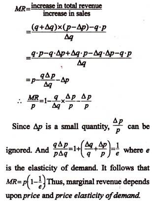
The relation among MR, AR and e_p may now be shown formally:

Proof:

MR = p (1 – 1/e_p)

Suppose q units of a commodity can be sold at price p and q + Δq units at a price p – Δp where Δq and Δp are very small quantities. Then marginal revenue

Equilibrium of a Monopolist in the Short Run:

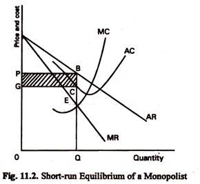
The objective of a monopolist like that of a competitive seller is maximisation of profit. This is achieved by equating MR with MC as is shown in Fig. 11.2.

In Fig. 11.2, AR be the demand curve for a monopolist’s product or the average revenue curve and MC is the marginal cost curve. AC shows the average cost. Since under monopoly MR is always less than price, the MR at each level of output will be shown by a downward sloping line lying below the AR curve. Let MR be the curve showing marginal revenue. MR and MC intersect at E.

Therefore, marginal cost and marginal revenue are equal when output is OQ. The average revenue curve shows that when output is OQ, the price is OP or QB. The monopolist will secure maximum net revenue when he produces OQ units. The monopoly price is QB.

The net monopoly revenue:

= total revenue – total cost

= OQ x QB-OQ x QC

= OQBP – OQCG = PBCG.

In Fig. 11.2, monopoly equilibrium is illus­trated on the assumption of rising marginal cost.

Monopoly Equilibrium under Constant Marginal Cost:

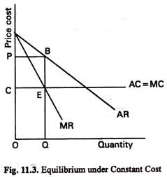
In Fig. 11.3, AR and MR are the average revenue and the marginal revenue, respec­tively. The cost curve is horizontal because the average and the marginal costs are, in this case, equal. E shows the point where MC and MR are equal. It follows that the equilibrium output is OQ. The price is QB or OP. Mono­poly profit is PBEC.

Monopoly Equilibrium under De­creasing Marginal Costs:

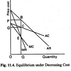
In Fig. 11.4, AR and MR are the average revenue curve and the marginal revenue curve, respectively. Under decreasing cost the average cost and the marginal cost slope downwards to the right. They are shown by QC and MC.

It has been proved that the marginal cost curve must be below the average cost curve. From the diagram we see that at E the MR and MC are the same. Therefore, the equilibrium output is OQ. The monopoly price is BQ or OP. The monopoly profit is PBCG.

In such a situation, the MC curve and the MR curve both slope downward to the right. Equilibrium can occur only if the relative position of the two curves are as shown in Fig. 11.4. In other words, there is equilibrium when the MC curve cuts the MR curve from above.

Factors Taken into Account by the Monopolist in Fixing Price:

The monopolist cannot directly control the price because the amount of a commodity which can be sold at a particular price depends on the market demand schedule. The mono­polist can, to a certain extent, influence demand, through advertisement and salesmanship, but on the whole the demand depends on con­sumers’ preferences over which the monopo­list has little control.

A monopolist, therefore, adjusts the supply (over the amount of which he has complete control) to that level which will maximise his net revenue. The first step taken by the monopolist is usually to fix the price. By a process of trial and error he finally fixes the amount to be produced.

The two most important factors which the monopolist has to take into account in fixing prices are:

(i) elasticity of demand and

(ii) the cost conditions.

1. Monopoly price and elasticity of demand:

If the demand is elastic, raising prices will reduce demand greatly. But, if demand is inelastic, prices might be raised considerably without reducing demand much. In the case of commodities with highly inelastic demand the monopolist may even destroy a part of the supply in order to get more revenue.

2. Monopoly price and cost conditions:

The monopolist must take into account his cost conditions. If the commodity is subject to diminishing returns, reduction of output will reduce marginal costs and may increase monopoly revenue. Under increasing returns, expansion of output will reduce marginal costs and may increase revenue. In the latter case the monopoly price may even be lower than the competitive price. It is, however, very much unlikely.

Monopoly Price in the Long Run:

In the short run and also in the long run, the monopolist will produce an output which will maximise his profit. The monopolist will earn maximum profit by equalising his MC with the MR.

In the long run the MR-MC rule applies in the sense that as long as output is positive, maximum profit is obtained by producing the level of output which corresponds to the equality between MR and MC.

However, the first rule of profit-maximisation (i.e., Q > O if P > AVQ has to be applied with minor modification. In the short run a firm will produce a positive quantity if TR = TVC. But in the long run a firm will produce anything at all if and only if all costs are covered, i.e., TR = TC. Here TC includes those that are fixed and those that are variable in the short run. In the long run all those costs are variable. Short-run excess profits do not dis­appear in the long run due to entry barriers.

In the short run the monopolist will operate on his short-run MC curve. In the long run the monopolist will operate on his MC curve. In the long run the monopolist will be able to reorganise the scale of production. Also there will be differences in the shape and position of the AR curve (demand curve) of the product between the short-run and the long-run.

In short, the profit maximisation formula (MR = MC) is applicable in both the short- and long-run monopoly price. The differences between the short and long monopoly price follow from the shape and position of the curves.

However, if a monopolist operates profitably in the short run, it will try to operate or a much larger scale in the long run. It may set up a new plant or increase the size of an exciting plant. In fact, a single plant mono­polist way because a multi-plant one.

The Total Revenue-Total Cost Approach:

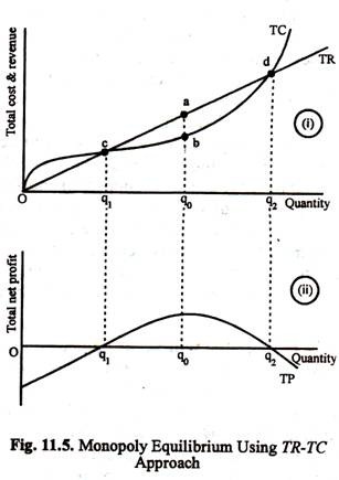
There are two ways of analysing the beha­viour of a profit-maximising firm. The first technique involves use of average cost and revenue curves. So long we have used the first technique in analysing monopoly equilibrium. We may now use the second technique to analyse monopoly situation in the long run. The alternative technique uses total revenue and total cost curves as shown in Fig. 11.5.

Profit is maximised by making the difference between TR and TC as large as possible. In Fig. 11.5 it happens at output q₀ where the vertical distance between the two curves is maximum. In lower part of the diagram we draw the curve of total (net) profit TP. Net profits are negative, if the monopolist pro­duces less than q₁ and more than q₂ units of output. Net profit is maximum at the output level q₀.

Monopoly Market # 3. Five Points about Monopoly Optimal:

Five important conclusions emerge from our discussion and analysis of monopoly equilibrium:

(i) A Monopolist can Control Either Price or Quantity:

A monopolist can control either price or quantity, though not both at the same time. It may be apparently seen that the mono­polist, being the only supplier of a commodity, can charge any price he likes. This is not true. It is because the monopolist has little, if any, control over consumers’ demand (although he has complete control over the supply of commodity). Since the demand curve of the monopolist is also the market demand curve for the product it is always downward sloping. The implication is obvious.

The monopolist is faced with two options:

(i) If the objective is to sell more, price cut is essential;

(ii) If the objective is to raise price, output restriction (or creation of an artificial shortage) is vital.

But the monopolist can never raise the price and force the buyers to buy more at this price. As R. G. Lipsey and C. Harbury have rightly commented: “If he (the monopolist) chooses to set price the quantity it will be able to sell is fixed by the demand curve. If he chooses to set output, the price, at which that output can be disposed off, is also fixed by the demand curve. The monopolist cannot-set both price and output”.

(ii) A Monopolist will Never Operate on the Inelastic Part of its Demand Curve:

It is to be noted that when demand for the product of monopolist is inelastic (e_p < 1), MR will be negative. Since MC is always positive MR- MC Equality will not be reached in such a situation. So the possibility of profit mini­misation is ruled out.

(iii) A Monopolist does not Always Earn Supernormal Profits:

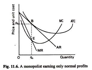
It may apparently seem that the monopolist always earns supernormal profits by creating artificial barriers to the entry of new firms. However, this is not the whole truth. In order to make excess profit a monopolist has to be efficient i.e., he has to produce a commodity at low cost. In Fig. 11.6 we observe that a monopolist is just able to make normal profit because ATC = AR = P at the profit-maximising output q₀.

It seems that the monopolist is a high-cost producer. In pure competition this break-even point is invariably reached by a firm in the long run due to freedom of entry and exit. In monopoly this is just a coincidence. It does not happen most of the time. Here the AR curve is just tangent to ATC curve at B. If the ATC curve lies uniformly above the AR curve the firm would even incur losses in the short run. It would stay in business in the short run if variable cost is covered. If this happens in the long run too, the firm would leave the industry and the commodity will not be produced.

(iv) A Monopolist Need not Necessarily Maximise Profit:

Monopolists often make super-normal profits. But this is not always the case. It is also wrong to suppose that if a monopoly firm is unable to make super­normal profit it will be making sub-normal profits.

In Fig. 11.2, we see that the monopolist is making excess profit of GCBP. But it is quite possible for the monopolist to produce a different level of output other than q₀ and still remain in business in the long run so long as TR > TC.

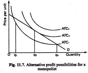
Profit maximisation implies that the monopoly is doing as well as it can do, given the cost and demand curves that it faces; it does not imply that profits are being earned. The monopolist faces a demand curve of D. Here we show three alternative cost curves. With the curve ATC₃, there is no positive output at which the monopolist can avoid making losses.

With the curve ATC₂, the monopolist is able to cover all costs at output q₂, where the ATC₂ curve is tangent to the average revenue (demand) curve. With the curve ATC₁, excess profits can be made by producing at any output between q₂ and q₃ (The profit-maxi­mising output will lie somewhere between q₂ and q₃ where MR = MC. This has not been shown on the diagram.)

(v) The MC Curve of the Monopolist is not the Supply Curve:

When a firm faces a downward sloping demand curve, there is no unique relation between the price that it charges and the quantity that it sells.

It is not possible to find out one-to-one relation between a particular price and quantity offered for sale at that price. So we cannot locate any point on the supply curve. Hence the supply curve cannot be drawn.

Monopoly Market # 4. Effects of an Increase in the Demand for the Product of a Monopolist:

An increase in the demand for the product of a monopolised commodity means that consumers are willing to pay more for the same quantity of the commodity than before. The demand curve has shifted upwards. Naturally the MR curve also moves upwards and intersects the MC curve at a higher point.

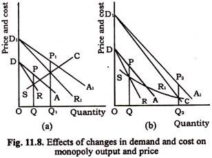
Since the monopolist will operate at the point where MC is equal to MR the new output will be larger than before. The price also will generally be higher but cases are conceivable where the price may be lower. These are illustrated in Fig. 11.8.

In Figure 11.8, SC is the marginal cost curve. DA and DR are the demand curves and the marginal revenue curves, respectively, before increase of demand, and D₁A₁ and D₁R₁ the demand curve and the marginal revenue curve after increase of demand.

Fig. 11.8(a) shows a monopoly operating under diminishing returns. In this case, when the demand curve rises from DA to D₁A₁ the output increases from OQ to OQ₁ and the price rises from QP to Q₁P₁.

Fig. 11.8(b) represents a situation where the marginal costs decline at the relevant outputs. In this case, when the demand curve rises from DA to D₁A₁ the total output increases from OQ to OQ₂ but price falls from PQ to P₂Q₂.

In both cases, the extent of change of output and prices depend on the slopes of the cost curve and the MR curve.

The effects of a fall in demand can be analysed in the same way by considering D₁R₁, as the original position of the MR curve and DR in the later position.

Monopoly Market # 5. Price Discrimination:

Definition and Classification:

Price dis­crimination refers to the practice of charging different prices from different buyers of the same commodity or service. This cannot be done under perfect competition but can be done under monopoly.

Three Possible Types of Price Dis­crimination:

1. Personal discrimination:

The monopolist can charge higher prices from buyers whose intensity of desire is large or whose ability to pay is greater.

2. Local discrimination:

Different prices may be charged from different localities.

3. Trade or use discrimination:

For diffe­rent uses the prices may be different. Thus, electricity is sold to factories at a much lower rate than that for domestic consumption.

When is Price Discrimination Possible?

According to A.C. Pigou, price discrimination is possible only if two conditions are satisfied:

1. The demand must not be transferable from the high priced market to the low priced market. If rich people do not buy deluxe editions but wait for cheap ones, personal discrimination in books is not possible.

2. The buyers of low priced articles must not be able to resell them in the high priced market. If industrial buyers of cheap electricity are allowed to resell it for direct consumption there can never be two prices for electricity.

When is Price Discrimination Profitable?

Ordinarily no monopolist will practice price- discrimination unless it is profitable for him to do so.

Price discrimination is profitable only if the following conditions are satisfied:

(1) The demand for the monopoly product can be split up into different markets.

(2) The elasticities of demand in the different markets are different.

(3) The cost of keeping the various markets separate is not large relative to the differences in the demand elasticities.

The second condition is vital. If the demand elasticities in the different markets are equal, there is no scope for price discrimination. But if they are different, the monopolist will gain by charging different prices in the different markets.

The price obtained by the monopolist in each market depends upon the output offered there and the shape of the average revenue curve in the market. At equilibrium (when maxi­mum profits are earned) certain relations must hold good between the different variables involved. These are explained below.

Conditions of Equilibrium under Discriminating Monopoly:

The discriminating monopolist has to decide the following problems:

(i) the total output he would produce,

(ii) the distribution of the output between the different markets, and

(iii) the price to be charged in each market.

Suppose there are two markets available to a monopolist, market A and market B:

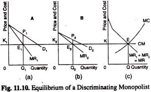
In market A his net revenue will be maxi­mum when the marginal revenue (at output q₁) is equal to K, his marginal cost. Similarly, in market B his net revenue is maximum when the marginal revenue (at output q₂) is equal to K. Therefore, at equilibrium, the marginal revenue in each market must be the same (both being equal to K, the marginal cost of producing the whole output).

If the marginal revenue in any market is greater than K, the monopolist increases his total revenue by selling more in that market. If the marginal revenue in any market is less than K, the monopolist is losing and must reduce his sales in that market.

Thus, at equilibrium, the following conditions must be satisfied:

I. The marginal revenue in all the markets must be equal.

II. The marginal revenue in each market must be equal to the marginal cost of producing the whole output.

The relationship between marginal revenue and price is given by the formula mr = p (1 – 1/e).

Using the symbols indicated earlier we get the following equation:

Marginal Revenue in market A = p₁ {1- 1 / r₁}

Marginal Revenue in market B = p₂ {1- 1 / r₂}

It has been shown that when the monopolist is earning maximum net revenue, the margi­nal revenues in the two markets must be equal.

Therefore, at equilibrium:

p₁ {1- 1 / r₁} = p₂ {1- 1 / r₂}

In this equation if e₁ = e₂ then p₁= p₂. Therefore, it follows that when the demand- elasticities (in the different markets, at the relevant output levels) are equal, the monopolist will charge the same price in the different markets. If the demand elasticities are different, price discrimination is profitable, and, there­fore, possible.

The relationship between the price in the two markets (p₁: p₂) can be calculated from the equation given above. In general, the price -will be higher in the market where the elasticity of demand is lower.

The analysis of price discrimination, given above, can be easily extended to the case of more than two markets.

The conditions of price-output equilibrium under discriminating monopoly is shown below:

In Fig. 11.10 (a), D₁ shows the average revenue and MR_X the marginal revenue in a market I. In Fig. 11. 10(b), D₂ shows the average revenue and MR₂ the marginal revenue in market II. These markets have different elasti­cities of demand at each price. Fig. 11.10(c); shows the combined marginal revenue earned from the two markets. The curve MR is obtained by adding the curves MR₁ and MR₂ horizontally, that is, MR₁ + MR₂ = MR.

MC shows the marginal cost curve of the whole output of the monopolist. The profit maximising output is shown by the intersection of MC and MR.

At equilibrium the output is OQ and marginal revenue is MR. Therefore, OK=MR. The line CM shows the marginal revenue and also the marginal cost. In market I the marginal revenue is OK₁ and price is P₁Q₁. Similarly, in market II, the marginal revenue is OK and price is P₂Q₂. The diagram shows that MR in all the markets must be same and the MR must also equal MC. It is also shown that MR₁, = MR₂ = MC.