Determining the Quantity of Output to be Produced | Monopoly

The below mentioned article will guide you about how the multi-plant monopolist would determine the quantity of output to be produced.

If the monopolist produces his product in more than one plant, then his organisation is called a multi-plant monopoly. We shall now discuss how the multi-plant monopolist would determine the quantity of output to be produced with a view to earning the maximum amount of profit.

For the sake of simplicity, we shall assume that the monopolist produces his output in only two plants. Let us first see how he would distribute the production of any particular quantity of output (q) between the two plants, so that the cost of production may be minimum. The total cost (C) of producing any particular quantity of output, q, is

C = C₁(q₁) + C₂(q₂) = C(q₁, q₂)                                  (11.22)

subject to q = q₁ + q₂ = constant                            (11.23)

where q₁ = quantity of output to be produced in the first plant, q₂ = quantity of output to be produced in the second plant, C₁ = cost of production in the first plant, and C₂ = cost of production in the second plant.

Here the first-order conditions (FOCs) of producing an output quantity, q₁ in the two plants at the minimum cost, i.e., the FOCs for minimising the cost of the output quantity q are

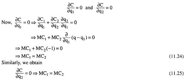
(11.24) and (11.25) give us that the monopolistic firm would distribute the production of any particular quantity of output (q) between the two (or more) plants in such a way that the marginal cost in each plant may become the same. We may easily understand the economic significance of this condition.

Instead of MC₁ being equal to MC₂, if we have MC₁ > MC₂ (in the two-plant case), then the firm would reduce the quantity of production in plant 1 and in­crease the quantity in plant 2, total output remaining the same, i.e., the firm would transfer production from the plant with a higher MC (here plant 1) to the plant with a lower MC (here plant 2). For, by doing this, it would be able to produce the same output (q) at a lower cost.

Now, the profit-maximising firm will produce at some point in the second stage of production where its MC curve would be upward sloping to the right. That is why, as it decreases q, and increases q₂, MC, will fall and MC₂ will rise, and, ultimately, at some distribution, MC₁ will become equal to MC₂.

This distribution is the cost-minimising distribution of q between the two plants. For, if MC₁ = MC₂, it will not be possible for the firm to reduce the cost further by transferring output production from one plant to the other.

On the other hand, if MC₁ < MC₂, the firm will reduce output in plant 2 and increase it in plant 1 till MC₁ rises and MC₂ falls to become equal to each other.

Thus, we come to the conclusion that the multi-plant monopolist will distribute the production of any particular quan­tity of output over his many (here two) plants in such a way that the MC in each plant may become the same; only then it would be able to produce the output at the minimum cost.

Therefore, that at each quantity of output, q, there is a problem of cost-mini­misation or profit-maximisation (the price, p, and, therefore, total revenue, p x q, being given by the demand curve). Here equilibrium will be obtained at that quantity, q*, at which profit is maximum among the maximums, or, maximum maximorum, as it is called.

We may now proceed to explain how the equilibrium output, q*, of a multi-plant monopoly with maximum maximorum of profit, is obtained. It follows from (11.24) and (11.25) that at any output q (= q₁ + q₂), the condition MC₁ = MC₂ ensures cost-minimising or profit-maximis­ing distribution of q between the two plants.

Now at any q = q₁ + q₂, the MC of the monopolist is MC₁ = MC₂. This is because here the qth unit of output is either the q₁th unit of output in plant 1 or the q₂th unit of output in plant 2 and the additional cost of producing that unit is either MC₁ or MC₂, and MC₁ = MC₂.

On the revenue side, the firm is a simple (non-price-discriminating) monopoly—it sells its product at a price given by its demand (or average revenue) curve.

Now, if at any q, the firm has MC = MC₁ = MC₂ < MR (marginal revenue), then it would be able to earn a positive profit on the margin, and so, it would increase its output to push up the level of profit.

But, as q increases, the MR, being a decreasing function of q, would diminish, and MC (= MC₁ = MC₂) would increase, since in the relevant range both MC₁ and MC₂ are increasing functions of q.

Therefore, q, while increasing, would eventually assume a value (say, q*) at which we would have MR = MC (= MC₁ = MC₂). At this q = q* the firm would earn the maximum maximorums of profit. For, now, its profit on the margin is zero, and so it will not be able to increase its profit by increasing q.

Similarly, if at some q, the firm has MC (= MC) = MC₂) > MR, then it would suffer losses on the margin, and so, it would now want to shed the loss-earning marginal unit(s), i.e., it would now want to decrease q to maximise its profit. But as q decreases, the firm’s MC (= MC) = MC₂) would also decrease and its MR would increase.

Eventually, at some q – q*, the firm would have MC (= MC) = MC₂) = MR, and this q = q* would be its q with maximum maximorum of profit. For, now, its losses on the margin are zero, and so it is no longer required of the firm to decrease its output in order to maximise profit.

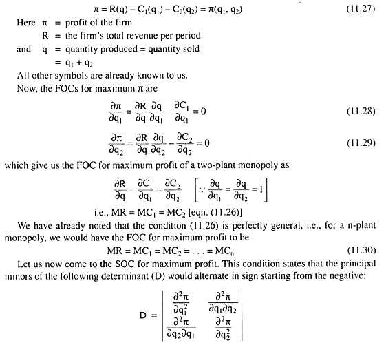
It follows from the above analysis that the necessary or the first order condition (FOC) for profit maximisation of a multi-plant monopoly is

MR = MC₁ = MC₂                         (11.26)

However, condition (11.26) is not the sufficient or the second order condition (SOC) of profit-maximisation. For if, at the MR = MC) = MC₂ point, the firm finds that a further increase in output would result in MC (= MC₁ = MC₂) being less than MR, which can, of course, happen in an inefficient stage of production, then the firm would not settle at this point, instead it would go on increasing its level of output, for by doing that, it would be able to increase its profit level.

Therefore, the SOC for profit maximisation states that at the point where the FOC is satisfied, i.e., at the MR = MC₁ = MC₂ point, further increase in output should result in MC = MC₁ = MC₂ being greater than MR. In that case, there would be a loss on the margin and so, the firm would not venture beyond the point (where the FOC is satisfied).

In other words, the second order condition for profit maximisation in a multi-plant monopoly states that at the point of intersection between the MC curve and the MR curve, i.e., at the point where the FOC has been satisfied, the slope of the MC curve, viz., the MC_{1 + 2} curve in Fig. 11.16, should be greater than that of the MR curve.

It may be noted that since the firm operates in the stage of efficient production, it would operate along the upward sloping portions of its MC₁ and MC₂ curves, and so the SOC would be automatically satisfied, for the MR curve of a monopoly is negatively sloped, by definition.

We shall now see how we may obtain the profit-maximising conditions of a multi-plant monopoly with the help of calculus. The profit (n) function of the two-plant monopoly under discussion is

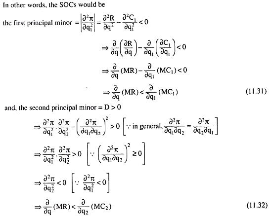
Eqns. (11.31) and (11.32) give us the SOCs for profit maximisation of a two-plant mo­nopoly. These conditions state, as we have already mentioned, that at the MR = MC₁ = MC₂ point, where the FOC is satisfied, the slope of the MR curve of the firm should be less than the slopes of both the MC₁ and MC₂ curves.

We have already mentioned the significance of this condition. Like the FOC, the SOC is also perfectly general. That is, for an-plant monopoly, it states that at the point where the FOC is satisfied, the slope of the MR curve should be less than the slope of the MC curve of each of the n plants.

We may now geometrically illustrate the price-out- put determination of a multi-plant (here two-plant) mo­nopolistic firm with the help of Fig. 11.16. In this fig­ure, we have shown the AR and MR curves on the one hand and the MC₁, MC₂ and MC_{1 + 2} curves on the other hand. The MC₁₊₂ curve is actually the MC curve of the multi-plant monopolist. It is obtained by laterally adding together the MC₁ and MC₂ curves.

This curve, along with the curves MC₁ and MC₂, would show us what is MC at any q and how this q should be divided between the two plants so that the MC at this q may itself become MC₁ = MC₂. For example, at q = q*, the MC of the firm is OT or Eq*.

Now if the production of q* of output is so distributed between the two plants that q* is produced in plant 1 and q₂ is produced in plant 2 (q* + q₂ = q *, by construction), then the MC in both the plants would be OT, i.e., here we would have: MC = MC₁ = MC₂ = OT.

In Fig. 11.16, the equilibrium point of the two-plant monopoly is the point E, which is the point of intersection of the MC₁₊₂ curve and the MR curve of the firm. For, at this point, i.e., at q = q*, we have

MR = MC₁ = MC₂ [eqn. (11.26)]

i.e., at this point, the FOC of profit maximisation has been satisfied. At q = q*, the SOC also is satisfied. For, at this output, the slope of the MR curve is nega­tive, and when q₁ and q₂ of this output are produced in the two plants, both MC₁ and MC₂ curves are positively sloped. That is, at q = q*, q₁ = q₁* and q₂ = q₂ (q* = q₁* + q₂), the slope of the MR curve is less than the slopes of the MQ and MC₂ curves, and the SOC is satisfied.