Concept of Relations and Functions | Optimization Technique

In this article we will discuss about the Concept of Relations and Functions.

Generally, graphs are used to find out the rela­tion between different variables, but when the rela­tions are complex, equations and computer simula­tions are more powerful tools. A relation is defined as given if for an x value, one or more y values will be specified by the relation.

As a special case, however, a relation may be such that for each x value there exists only one cor­responding y value. In that case y is said to be a function of x, and that is denoted by y — f(x), which is read: y equals f of x [Note: f(x) does not mean f times x]. A function is therefore a set of (x, y) with the property that any x value uniquely determines a y value. A function must be a relation but a relation may not be a function.

In the function y = f(x), x is referred to as the argument of the function and y is called the value of the function. Alternatively, we refer to x as the inde­pendent variable and to y as the dependent variable.

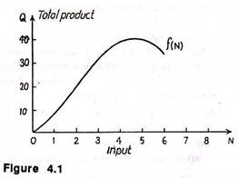
Let N denotes the input of variable resources per unit of time, and Q denotes the total product pro­duced per unit of time corresponding to the different levels of N.

Q = f (N) (4.1)

Such a production function is represented by the data given in table (4.1).

It may be possible to express the function by means of an equation such as:

Q = 2N^0.5 or Q = 5 + 8N – 2N²

From which values of Q can be calculated for specific values of N. In fig. (4.1), we have shown table (4.1) graphically.

All three methods of expressing relations—(i) ta­ble, (ii) graph and (iii) equation play an important role in decision making.

Total, Average and Marginal Relations:

In optimization analysis, total, average, and mar­ginal relations are very useful. The definition of to­tal and average are well known, but the definition of marginal needs explanation. A marginal is deemed as the change in the dependent variable of a func­tion associated with a unitary change in one of the independent variables.

Table (4.2) shows the relation between totals, av­erage and marginal for a hypothetical production function.

(AP_N) = Total physical product per period/Units of input used per period

2. Marginal Product (MP/_N) = Difference be­tween successive figure in total physical product per period (col. IV).

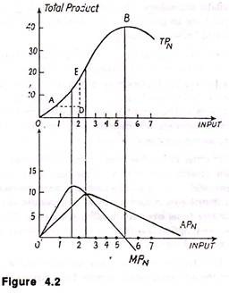
Table 4.2 can be plotted graphically to show the relation between total, average and marginal fig. 4.1(a) and (b).

i. Average Product:

This is defined as (AP_N) = _Q/N

Thus (AP_N) at point A on the graph is 7 units. This is the slope of the ray OA which connects point A with the origin. (AP_N) at B is exactly the same since it lies on the same ray through the origin (39.9/ 5.7 = 7).

ii. Marginal Product:

If Δ is used to show a small change, so that ΔQ is a change in Q and ΔN is a change in N, then marginal product is defined as:

This is the average slope of the total product curve itself over the interval. For instance (MP_N) for the second unit of input is the slope of the line AE which equals:

ED/AD = 13/1 =13

At a given point, however, (MP) is the actual slope of the total product curve.

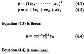
Non-Linear Functions:

Generally, linear graphs and equations are used to illustrate economic relationship. Some of the com­mon non-linear relationships we often come across in economics are shown below:

In fig. 4.3(a), (b), (c) the value of y depends on constant term and value of x, x² and x³ respectively. In the rectangular hyperbola noted in fig. 4.3(d), the curve is asymptotic to both the axes (the curve does not touch the axes).

In fig. 4.3(e) expotentional graph is shown which is used to explain growth in economics. Fig. 4.3(f) shows a logarithmic function. In decision-making a dependent variable y may be a function of more than one independent variable. For example, total product is a function of labour, capital, fuel, business organisation, etc.

When y is a function of more than one variable, we express it as:

To express the above function graphically we need many axes and the figure gets not only complex but very cumbersome to draw. Even without draw­ing these functions we can work out the average and marginal. To work out the marginal, concept calcu­lus is essential. In the section to follow we give a short and precise exposition of differential calculus.