Law of Equi-Marginal Utility (With Diagrams)

Read this article to learn about the Law of Equi-Marginal Utility or the Principle of Substitution.

In the real world, a consumer may purchase more then one commodity. Let us assume that a consumer purchases two goods X and Y. How does a consumer spend his fixed money income in purchasing two goods so as to maximize his total utility? The law of equi­-marginal utility tells us the way how a consumer maximizes his total utility.

Before elaborating this law, let us assume:

a. The consumer acts rationally.

b. Tastes and preferences, money income, prices of goods, etc., remain constant.

The equi-marginal principle is based on the law of diminishing marginal utility. The equi-marginal principle states that a consumer will be maximizing his total utility when he allocates his fixed money income in such a way that the utility derived from the last unit of money spent on each good is equal.

Suppose a man purchases two goods X and Y whose prices are P_X and P_Y, respectively. As he purchases more of X, his MU_X declines while MU_Y rises. Only at the margin the last unit of money spent on X has the same utility as the last unit of money spent on Y and the person thereby maximizes his satisfaction.

Only when this is true, the consumer will not be distributing his money in buying good X and Y, since by reallocating his expenditure he cannot increase his total utility.

This condition for a consumer to maximize utility is usually written in the following form:

MU_X/P_X = MU_Y/P_Y

So long as MU_Y/P_Y is higher than MU_X/P_X, the consumer will go on substituting Y for X until the marginal utilities of both X and Y are equalized.

The marginal utility per rupee spent is the marginal utility obtained from the last unit of good consumed divided by the price of good (i.e., MU_X/P_X or MU_Y/P_Y). A consumer thus gets maximum utility from his limited income when the marginal utility per rupee spent is equal for all goods.

Example:

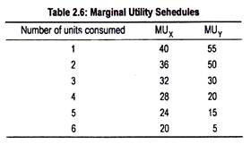
This equi-marginal principle or the law of substitution can be explained in terms of an arithmetical example. In Table 2.6, we have shown marginal utility schedule of X and Y from the different units consumed. Let us also assume that prices of X and Y are Rs. 4 and Rs. 5, respectively.

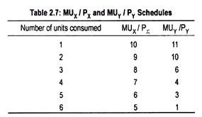
MU_X and MU_Y schedules show dimini­shing marginal utilities for both goods X and Y from the different units consumed. Dividing MU_X and MU_Y by their respective prices we obtain weighted marginal utility or marginal utility of money expenditure. This has been shown in Table 2.7.

MU_X/P_X and MU_Y/P_Y are equal to 6 when 5 units of X and 3 units of Y are purchased. By purchasing these combinations of X and Y, the consumer spends his entire money income of Rs. 35 (= Rs. 4 x 5 + Rs. 5 x 3) and, thus, gets maximum satisfaction [10 + 9 + 8 + 7 + 6] + [11 + 10 + 6] = 67 units. Purchase of any other combination other than this involves lower volume of satisfaction.

Graphical Representation:

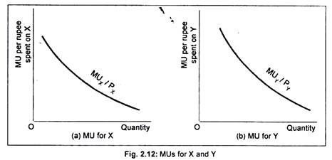
The above principle can also be illustrated in terms of a figure. We have drawn marginal utility curves for goods X and Y in Fig 2.12(a) and (b).

Here we use marginal utility and price. Marginal utility per rupee spent on good X = MU_X/P_X, and that of Y = MU_Y/P_Y. The MU_X/P_X curve has been shown in Fig. 2.12(a) while the MU_Y/P_Y curve has been shown in Fig. 2.12(b). We have not drawn negative portion of the marginal utility curves.

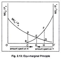
Now, by superimposing Fig. 2.12(b) on Fig. 2.12(a), we get Fig. 2.13 in which we measure available income—00’—of the consumer on the horizontal axis.

As we move rightwards from ‘O’, amount spent on X increases and, as we move leftwards from ‘O’, amount spent on Y increases. How does our consumer allocate his total income in buying both goods X and Y is described by equalizing per rupee spent on both?

Our consumer maximizes his total utility by spending OD amount on good X and O’D amount on good Y. By purchasing this combination, the consumer equalizes marginal utilities per rupee spent on X and Y at point E (i.e., MU_X/P_X = MU_Y/P_Y = ED). No other combination will give greater satisfaction.

If our consumer spends OC on good X and O’C on good Y then MU_X/P_X will exceed MU_Y/ P_Y by the distance AB. This will induce the consumer to buy more of X and less of Y. As a result, MU_X/P_X will fall, while MU_Y/P_Y will rise until equality is restored at point E. Similarly, if the consumer spends OH on X and O’H on Y then MU_X/P_X< MU_Y/P_Y. Now, the consumer will buy more of Y and less of X.

This substitution between X and Y will continue until MU_X/P_X= MU_Y/P_Y. Therefore, the consumer can derive maximum satisfaction only when marginal utility per rupee spent on good X is the same as the marginal utility per rupee spent on another good Y. When this condition is met, the consumer does not find any interest in changing his expenditure pattern.

The equilibrium condition can now be rewritten as:

MU_X/P_X= MU_Y/P_Y

This equation can, however, be rearranged in the following form:

MU_X/MU_Y = P_X/P_Y

This equation states that a consumer reaches equilibrium when he equalizes the ratio of marginal utilities of both goods with the price ratio.

However, this equilibrium condition can be extended to ‘n’ number of commodities.

For ‘n’ number of commodities, the equilibrium condition is:

MU_A/P_A= MU_B/P_B= MU_C/P_C = ……… = MU_n/P_n

Limitations:

This law of substitution has been criticized on the following grounds:

Firstly, the law of equi-marginal utility is based on the measurability of utility in cardinal numbers. But utility is a subjective concept and, hence, not quantifiable.

Secondly, this law assumes that the consumer acts rationally. No consumer, in fact, purchases commodity in accordance with this principle of substitution. In fact, purchases are often guided by habit, sentiment, prejudice, or custom.

Thirdly, this law cannot be applied in the case of indivisible commodities like motor car, refrigerator, etc. Since these commodities are not divisible into smaller units, the law may seem to be inoperative.

Derivation of Demand Curve from Equi-Marginal Utility:

In order to be able to derive the demand curve for a commodity we must know the equilibrium purchase plan of a consumer of various commodities.

We want to know the equilibrium purchase of commodities because the basic aim of a consumer is the maximization of satisfaction from the consumption of various commodities. The equilibrium of the consumer may be explained in terms of the law of equi­-marginal utility or the law of substitution.

This law states that a consumer will be maximizing his satisfaction from the expenditure of his limited money income when the marginal utility per rupee spent on, say, one good, X, is the same as the marginal utility of rupee spent on another good, Y. In other words, a consumer reaches equilibrium when the marginal utility per rupee of good X (MU_X/P_X) is equal to the marginal utility per rupee of good Y (MU_Y/P_Y).

Symbolically, the principle of equi-­marginal utility or the condition for equilibrium of a consumer can be written as:

MU_X/P_X= MU_Y/P_Y

Or MU_X/MU_Y = P_X/P_Y

This equation tells us that the consumer obtains maximum satisfaction from the consumption of goods X and Y from his limited income when the ratios of marginal utilities are equal to the price ratios for each goods consumed.

This equilibrium condition can be used for the derivation of the demand curve for one good, say X. To derive the demand curve for X, we assume that tastes, money income and prices of other goods, say Y, remain constant. Suppose the consumer is in equilibrium when

MU_X/P_X= MU_Y/P_Y

Now the price of X falls to P_X1.

The consumer will be out of equilibrium, i.e.,

MU_X/P_X1 > MU_Y/P_Y

To restore equilibrium, the consumer must buy more of X and less of Y. Therefore, MU_X must fall because of the hypothesis of diminishing marginal utility. As the consumer purchases more of X he must buy less of Y. Consequently, MU_Y will rise. As a result, the left side of the equilibrium condition has become larger while the right side has become smaller.

The consumer, thus, does not reach equilibrium. To reach equilibrium, the consumer transfers his given money income from Y to X, that is, buy more of X and lowers its marginal utility and buy less of Y and raises its marginal utility. This process will continue until equality is restored, i.e.,

MU_X1/P_X1 > MU_Y1/P_Y1

What we have thus seen is that a fall in the price of a good, ceteris paribus, leads to an increase in its demand. Thus, the demand curve for the commodity in question is negative sloping.

The Paradox of Value:

We know that a consumer reaches equilibrium when marginal utility for a commodity, say X, is equal to its price, i.e., MU_X = P_X. Thus, there is a link between price and MU, rather than price and total utility. Price of a commodity is determined in accordance with its MU, instead of total utility.

Earlier economists could not explain why the price of water is so less though its total utility is great and why the price of diamond is so high though it has virtually no utility. This problem came to be known as the paradox of value. It was Marshall who resolved this paradox with the aid of the concept of MU.

Water is available almost in plentiful amount. Its MU is thus low because of its abundance.

As its MU is low, the price of water is low. On the other hand, the supply of diamond is scarce in relation to demand. Though its total utility is comparatively less, its MU is too high because of scarcity. So its price is high. Thus, the value or price of a commodity depends not on its total utility but on marginal utility and availability of commodity.