Keynesian Consumption Function: A Close View

The below mentioned article provides a close view on Keynesian consumption function.

The consumption function states that aggregate real consumption expenditure of an economy is a function of real national income. This is called the Keynesian Consumption Function. The classical economists used to argue that consumption was a function of the rate of interest such that as the rate of interest increased the consumption expenditure decreased and vice versa. Keynes stated that the rate of interest may have some influence on consumption but the real income was the important determinant of consumption.

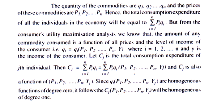
It should be remembered that in the consumption function consumption expenditure refers to intended or ex-ante consumption and not actual consumption. Similarly, income refers to anticipated income and not actual income. Therefore, the consumption function shows what consumption expenditure would be at different levels of income. The aggregate consumption in the economy can be found out from the consumption expenditure of different individuals purchasing commodities.

 

This means that, when all prices and the level of income change in the same proportion, the consumption expenditure will also change in the same proportion. If we write all prices as P and all money incomes as Y_m, then we can write that C_m = C_m (Y_m, P) where C_m is the aggregate consumption expenditure in money terms. This function will also be homogeneous of degree one in Y_m and P.

Thus, the aggregate consumption function states that real consumption is a function of real income and then the consumption function can be written as C = C(Y) where C is real consumption expenditure and Y is real national income. This is the Keynesian Consumption Function. The straight line consumption function has a constant slope at all points. The (MFC) marginal propensity to consume decreases as income increases.

According to Keynes the consumption function must possess the following characteristics:

(1) Aggregate real consumption expenditure is a stable function of real income.

(2) The marginal propensity to consume (MPC) or the slope of the consumption function defined as dc/dY must lie between zero and one i.e. 0 < MPC < 1.

(3) The average propensity to consume (APC) or the proportion of income spent on consumption defined as C/Y should be decreasing as income increases. From the relation between marginal and average we know that, when average falls, marginal is below average. Thus, when the average propensity to consume (APC) falls, the marginal propensity to consume (MPC) must be lower than the APC.

(4) The marginal propensity to consume (MPC) itself probably decreases or remains constant as income increases.

These four characteristics specify the shape of the consumption function. It can be seen clearly that, if we draw a straight line consumption function with a positive intercept with the vertical axis, and intersecting the 45° line from above, it will satisfy all the four characteristics. In Fig. 12.1 we draw Y on the horizontal axis and C on the vertical axis.

The consumption function, PQ, is a straight line and OT is a straight line passing through the origin making an angle of 45° which intersect the consumption function from below at point T. This consumption function PQ satisfies all the four characteristics.

(i) It represents a stable relationship between C and Y.

(ii) The slope of the line PQ represents the marginal propensity to consume (MPC) which has a positive slope. Again the consumption function cuts the 45° line from above. This means consumption function (PQ) is flatter than the 45° line and its slope is less than 45° line. The slope of PQ = MFC and the slope of the 45° line = tan 45° = 1. Thus, it satisfies the second characteristic that 0 < MPC < 1.

(iii) But the average propensity to consume will be different at different points of the consumption function. For example, at point P, C = OP and Y = 0, so that, APC = C/Y = OP/O = ∞.

It means at point P, the APC is infinity (∞). Again consider the point T where consumption is TS and income is OS, so that, APC = TS/OS = slope of OT = 1. Thus, APC at point T is one. The APC at any point on the consumption function is slope of the line joining that point with the origin. To the left of T, the AFC is greater than one and to the right of T, AFC is less than one. It means, to the left of the point T consumption is greater than income i.e., C > Y, so that, APC = C/Y > 1.

On the other hand, to the right of the point T, consumption is less than income, i.e. C < Y, so that, APC = C/Y < 1. Thus, the APC decreases as we move along the consumption function from left to right. Since the average propensity to consume (APC) decreases as income increases the marginal propensity to consume (MPC) must be less than the average propensity to consume. Thus, the third characteristic is also fulfilled by this straight line consumption function.

Fourthly, if the consumption function is a straight line the slope of the consumption function is constant at all points, i.e. the constant MFC satisfies the fourth characteristic. If the MFC is to decrease as income increases the consumption function has to be non-linear. It will be concave to the horizontal axis. In other words, the equation of a straight line linear consumption function can be written as C = a + bY, where a and b are constants. Let us also assume that a > 0 and 0 < b < 1 and dc/dY = b = MPC. Since b > 0, the function is upward rising. Again the APC = C/Y = a/Y + b. In this case, C/Y will decrease as Y increases. So the APC = C/Y = a/Y + dc/dY = MPC + x. .^.. APC > MPC.

These four characteristics of the consumption function mentioned by Keynes were not derived from theoretical analysis or empirical evidence. He derived these proportions from intuition. Keynes called it a “fundamental psychological law” that people do not spend the entire amount of the increase in income and save a part of it. This means that, marginal propensity to consume (MPC) is positive but less than one. The consumption income ratio falls as income increases which means that there is a non-proportional relationship between consumption and income.

Subjective and Objective Factors Affecting Consumption Expenditure:

According to Keynes, aggregate real consumption expenditure depends on aggregate real national income, other things remaining constant.

The factors other than the level of income that affect consumption can be divided into three groups:

(a) Subjective,

(b) Objective and

(c) Structural.

Subjective factors are psychological ones that cannot be quantitatively measured. Objective factors are considered to be economic variables that can be measured quantitatively. Structural factors include aspects particularly relevant for the problem of aggregation. Let us first consider the subjective or psychological factors affecting consumption.

The subjective factors consist of basic values, states of mind, attitudes, etc., which cannot be measured in quantitative terms. Keynes discuss the various motives for saving, such as, precaution, foresight, enterprise, pride and avarice; and also the motives-for consumption, such as, “enjoyment, short-sightedness, generosity, miscalculation, ostentation and extravagance.” He called them subjective factors that are unlikely to change significantly in the short-run.

Psychological factors, such as, expectations and attitudes do influence consumption. Rational behaviour suggests that a consumer who expects an increase in income or in price level would consume more than one who expects no such changes. Keynes accepted this logic but felt that expectations can be ignored because different people in an economy will have different expectations, and such expectations will probably cancel out each other in the aggregate analysis.

Now, let us consider the objective factors. The first objective factor after income is the interest rate. A rise in the interest rate may affect aggregate consumption expenditure in various ways. For example, a rise in the rate of interest will reduce bond prices, thereby discouraging the consumption propensities of the bondholders.

It may also have the effect of substituting one type of asset for another. Classical economists used to believe that, consumption or saving was primarily a function of the rate of interest. However, Keynes did not consider the interest rate to be an important factor in influencing consumption or saving.

The second factor influencing consumption expenditure is the volume of wealth. The argument is that, everything being equal, the more savings a man has, the less would be his desire to accumulate more. For example, if two persons have identical needs, tastes and incomes, but one has acquired a large fortune, his incentive to accumulate more will be less than the other person’s desire to accumulate wealth.

This means that if a person has already a great volume of wealth his propensity to consume will be high. This is also true for the whole economy. The greater the volume of wealth in the economy the greater will be the consumption expenditure. This is known as the Pigou effect.

A part of wealth is also held in the form of money. Any change in money holdings without an equivalent change in other wealth would be regarded as wealth effect. More money means more spending. It should be remembered that consumption expenditure depends on the real quantity of money and not on nominal quantity of money.

Thus, if the nominal quantity of money remain the same but the price level changes, there will be a change in the real quantity of money, which will change consumption expenditure. This is known as real balance effect. The third factor affecting consumption expenditure is the terms of consumer credit which have been considered to have significant affect on purchases of consumer durables. The less restricted the terms of credit, the greater will be the demand for consumer durables. However, the impact of consumer credit on the volume of consumption expenditure is difficult to measure.

The last but not the least, the sales effort of the producers would affect consumption expenditure. The sales effort through advertisement has a sig­nificant effect on the consumption expenditure. Other things remaining the same, the greater the volume of advertising expenditure greater will be the consumption expenditure.

Now, we wish to consider the structural factors affecting consumption. The first important structural factor is income distribution. We know that the marginal propensity to consume of low income people is substantially higher than the marginal propensity to consume of high income people.

Hence, when there is redistribution of income from rich income groups to poor income groups, this will increase consumption expenditure in an economy even if the level of income remains unchanged. This is because the loss of consumption of the rich people will be over-compensated by the gain of consumption of the poor since the marginal propensity of the poor is higher than the rich. Since the distribution of income changes slowly, it is unlikely to have a short- run impact in the economy at all.

When considering cross-section studies of consumption expenditure -we find that at any given income level there are significant differences between the consumption spending of different families. These differences can be explained at least partly, by demographic factors, such as family size, place of residence, home ownership, stage in the family life cycle and so on.

Other things remaining the same, spending of big families must be greater than that of smaller families. Rural families spend less than urban families. Families with young children are likely to spend more than without small children. These demographic factors are unlikely to change in the short-run and hence can be ignored in the short-run analysis. The fiscal policy can also influence the aggregate consumption expenditure.

If the government raises more money through taxation, it will reduce the disposable income and hence the consumption expenditure will fall. Similarly, if the government reduces taxes or make more transfer payments, the disposable income will increase and hence the consumption expenditure will also increase. Even if the national income remains unchanged, disposable income may change because of the fiscal operation of the government and, thereby, may change consumption expenditure as well.

The financial policies of the large corporations may also change the aggregate consumption expenditures. The dividend policies of large joint stock companies may increase or decrease income and thereby may change the consumption expenditure. Corporate savings may reduce disposable income of consumers and hence consumption expenditure at any level of national income.

Alternatively, if the corporations keep a large fraction of their income in the form of undistributed profits, this may discourage consumption expen­diture, or if the corporations give away a large fraction of their incomes in the form of dividend the consumption expenditure may increase.

We can conclude by saying that, there are many subjective, objective and structural factors which may influence consumption expenditure, but most of these factors remain unchanged in the short-run, and hence the short-run aggregate consumption expenditure may be regarded as a function of income. When any of these factors that are assumed to remain constant change, the consumption function will shift as well.

Empirical Support for the Consumption Function:

The Keynesian consumption function hypothesis was based neither on any theoretical foundation nor on any statistical study. It is mainly based on intuition. Two types of data may be used to test the validity of Keynesian hypothesis. One is budget studies data and the other is time series data. In the budget studies data we have information on consumption and income of families of different income groups within a year.

In the time series data we have information on total consumption and total income for a number of years. Keynes consumption function hypothesis has received support from the different budget studies and time series data. The earlier studies indicated that, the Keynesian consumption function is a good approximation of how consumers behave.

The cross-section budget studies involve taking a sample of households and classifying them according to their income groups. Divide the average level of consumption spending for each income group by the corresponding average level of income give each group’s average propensity to consume (APC). It has been found that the APC has a marked tendency to fall as we move from lower to higher income groups; also, the APC is greater than the MPC (Marginal Propensity to Consume) in every case. This is a typical result and supports the ‘absolute income’ hypothesis.

The study also reveals that households with higher income consume more, which implies that the marginal propensity to consume (MPC) is positive. These studies also found that households with higher income save more, which implies that MPC < 1. These data supported Keynes’s prediction that, the MPC lies between zero and one. In addition, studies also found that, higher- income households save a larger fraction of their income, which confirmed Keynes’s proposition that the APC falls as income rises.

Other studies examined aggregate time series data on consumption and income for the period between the two World Wars. These datas also supported some of the propositions of Keynesian consumption function. During these years income was usually low and thus, consumption and saving were low, indicating that, the MPC lies between zero and one. In addition, during those years of low income, the ratio of consumption to income was high, thus confirming Keynes’s second proposition.

Finally because the correlation between income and consumption was so high that no other variables appeared to be important for explaining consumption and thus, income appears to be the primary determinant of consumption. Thus, the Keynesian consumption function has been supported by time-series data as well.

Simon Kuznets: The Consumption Puzzle:

Short-run time series studies and household data found a relationship between consumption and income similar to the one proposed by Keynes. But studies of long-run time series found that the APC did not vary systematically with income. This long-run consumption function has a constant APC, whereas the short-run consumption function has a falling APC.

The results of this study do not support the ‘absolute income’ hypothesis as outlined above. Further, the long-run consumption function is found to be proportional as shown in Fig. 12.3. The ‘absolute income’ hypothesis appears to explain the cross-section and short-run time series data well, but fails to explain the long-run time series data. One objective of the more recent theories has been to try and reconcile this apparent conflict in the different sets of statistical results.

The Consumption Ratchet:

According to Dussenberry, the consumption function is irreversible with respect to the fall in income. This means that the consumption function applicable to the rise in income but inapplicable to the fall in income because, when income rises people become used to the high level of consumption and it becomes difficult to reduce consumption when income falls. For example, suppose that as income of an individual increases by £200, consumption increases by only £140. This phenomenon is known as the “Consumption Ratchet”.

The ratchet idea can be explained as follows:

During the long-term growth of income, the consumption function shifts in the upward direction. This upward shift normally occur during periods of relatively high income. Such shifts are irreversible during subsequent declines of income. Each shift “takes-off” from a platform provided by the previous peak. This gives the source of the ratchet effect.

The Saving Function:

The saving function can be deduced from the consumption function. Saving (S) is defined as the difference between income and consumption, i.e. S = Y – C = Y – C(Y). It means that saving (S) is a function of income, i.e. S = S(Y). The saving function can be known from the consumption function. The average propensity to consume is S/Y and the marginal propensity to consume is dS/dY, change in saving when income changes.

The saving function has the following characteristics:

(1) Saving is directly related to income, i.e. ds/dY > 0. Further, the Marginal Propensity Save (MPS) lies between 0 and 1, i.e. 0 < ds/dy < 1.

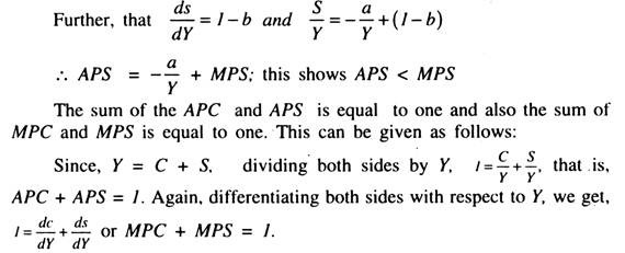
(2) Average Propensity to Save (APS) increases as income increases. This means that MPS is greater than APS. If consumption is a linear function of income, the saving function will also be a linear function of income. If the consumption has a positive intercept with the vertical axis the saving function will have a negative intercept with the vertical axis.

The saving function has four characteristics as the consumption function has four characteristics.

The four characteristics of saving functions are given as follows:

(1) Saving is a stable function of income,

(2) The marginal propensity to save lies between zero and one,

(3) The average propensity to save is directly related to income,

(4) The marginal propensity to save remains constant or increases as income increases. The consumption function and the saving function are both linear or non-linear. However, if the consumption function is concave from below, the saving function is convex from below.

By taking the vertical differences between the 45° line and the consumption function we get the saving function as in Fig. 12.2, when K = 0, consumption expenditure is equal to OP, which means that saving is equal to 0P'(— OP). When the level of income (Y) is OB, consumption equals income and, hence, the saving is nil.

To the left of B saving is negative as income is less than consumption and, to the right of B, income is greater than consumption and, therefore, saving is positive. Thus, we get the saving function P’Q’ from the consumption function PQ. The slope of the saving function is the MPS like the slope of the consumption function which is the MPC. If the saving function is a straight line, its slope will be the same at all points.

The average propensity to save at any point with the origin, for example at point D on the saving function, the APS is equal to the slope of the line OD = tan α, whereas the MPS is equal to tan β. Since β is greater than α, tan β is also greater than tan α, i.e. MPS > APS. This means that APS increases as income increases. When the consumption function is a straight line, its equation can be written as C = a + bY, where a and b are parameters.

Now, S = Y – C = Y – a – bY = -a + (1 – b)Y which means that the saving function is also a straight line with a negative intercept with the vertical axis -a and a slope is equal to (1 – b) which lies between 0 and 1, i.e. 0 < 1 – b < 1.

Thus, if we know one we can get the other. Again, if the consumption function is proportional the saving function is also proportional. The propor­tional consumption function can be written as C = bY. In this case, the saving function can be written as S = Y – C = Y – bY = (1 – b)Y.

It can be seen that the saving function is also proportional. If consumption is proportional to income, the consumption function will be a straight line passing through the origin. So will be the saving function. In that case, the APC = MPC and APS = MPS. Thus, in the long-run, the consumption function and the saving function will be straight lines through the origin as shown in Fig. 12.3.

Paradox of Thrift:

The simple prediction that equilibrium national income is decreased when the desire to save rises and increased when the desire to save falls, has been called the paradox of thrift. It is no paradox at all. It is really a simple prediction of a model in which national income is demand-determined. More saving means less spending and, thus, reduces the aggregate demand. Less saving means more spending and this means an increase in aggregate demand.

Let us assume that both investment and saving are functions of income and that the MPS is greater than the marginal propensity to invest. The investment function will then intersect the saving function from above. Now we assume that the saving habits have changed and people become more thrifty than before.

The result will be more saving at each level of income which means that the saving function will shift to the left and the effect of such a shift on the equilibrium level of income and on the volume of saving can be shown in the figure. In Fig. 12.4, as the saving function shifts to the left from S(Y) to S'(Y) the volume of saving is reduced from AB to CD. Thus we get the paradoxical result which can be explained as follows.

Firstly, it can be explained from the logical point of view that, what is true for each individual taken in isolation may not be true for all individuals taken together. To argue that what is true for individual must also be true for the aggregate is fallacious and is known as the fallacy of composition. Thus, it could be true that, when each individual saves a higher percentage of income, total saving may be less.

Secondly, we can also explain the paradox from the economic point of view. We know that the saving is a function of income. We also know that the equilibrium level of income is reduced when there is a leftward shift of the saving function. Thus, when the propensity to save increases, it reduces the level of income from OB to OD.

Since the level of income is reduced, the volume of saving also comes down automatically. Hence, the lower aggregate saving is the result of decrease in income, which is the result of the higher saving propensity. For example, suppose originally the saving propensity of the people was 0.2 and the equilibrium level of income was 200.

The total saving was 40. Now suppose the propensity to save has increased to 0.3. This means that the saving function shifts to the left and the equilibrium level of income fall to 100. At this level of income (100) total saving is 30. Thus, even if the saving propensity increases, total saving decreases — due to the fall in the level of income.

The paradox of thrift is an important factor to consider in an economy. In the Keynesian model we see that, as the saving propensity increases, the equilibrium level of income decreases. It points out that saving is an undesirable element as it lowers the level of income. If saving is undesirable how can we ask the developing countries to save more? Is the paradox of thrift applicable to the developing countries?

In the Keynesian model of income determination we assume that the economy is an advanced capitalist economy in depression where substantial unemployment exists, because of lack of effective demand. In such an economy there are idle capital goods which can be used if the effective demand can be increased. The increase in effective demand will increase income and employment. Supply of output in such an economy is highly elastic and demand-determined. But the situation is different in a developing economy.

In a developing economy,-unemployment is not caused by a deficiency in effective demand. It is a result of the low quantity of capital goods to work with. Employment cannot be increased because of lack of capital goods. Unlike unemployment in a developing economy which cannot be reduced by increasing total spending.

Since supply of output is inelastic in a developing economy an increase in spending will only lead to an increase in the price level. In a developing economy, more capital goods should be employed to increase income and employment. More capital goods can be obtained only through capital formation in a developing economy. Thus, it is only through saving that the level of income and employment can be increased in such an economy. It is clear from this analysis that the same prescriptions are not applicable in different economies where objective conditions are different.

While a capital formation approach is needed in a developing economy, a spending approach may be applicable in an advanced economy. This analysis also shows that, the Keynesian theory is inapplicable in a developing economy. Conclusions derived from the Keynesian theory are relevant for a developed economy and not applicable in a developing economy.

It needed to explain how these two consumption functions could be consistent with each other. Franco Modigliani and Milton Friedman each proposed explanations of these seemingly contradictory findings. But before we see how Modigliani and Friedman tried to solve the consumption puzzle, we need to discuss Irving Fisher’s contribution to consumption theory. Both Modigliani’s life-cycle hypothesis and Friedman’s permanent income hypothesis rely on the theory of consumer behaviour proposed by Fisher.

Irving Fisher and Inter-Temporal Choice:

When people decide how much to consume and save, they must consider both the present and the future. The more consumption they enjoy today, the less they will be able to enjoy tomorrow. In making this tradeoff, households must look ahead of their expected future income and to the consumption of goods and services they could afford.

Fisher developed the model with which economists analyze how rational, forward-looking consumers make inter-temporal choices — that is, choices involving different periods of time as Fig. 12.5 shows. Fisher’s model shows the constraints consumers face and how they choose consumption and saving.

The Inter-Temporal Budget Constraint:

Everyone would prefer to increase the quantity of goods they consume. The reason they consume less than they desire is that their consumption is constrained by their income, which is called budget constraint. When they are deciding how much to consume today and how much to consume tomorrow, they face an inter-temporal budget constraint. To understand how people decide their level of consumption, we need to examine this constraint.

We examine the decision facing a consumer who lives for two periods. Period one represents the consumer’s youth and period two represents the consumer’s old age. The consumer earns income of Y₁ and consume C₁ in period one, and earns income of Y₂ and consumes C₂ in period two. Because the consumer has the opportunity to borrow and save, C in any one period can be either greater or less than Y in that period. Consider how the consumer’s Y in the two period’s constraints C in the two periods.

In period 1, S₁ = Y₁ – C₁, where S is saving. In period 2, C equals the accumulated S, including the interest earned on the S, plus period II’s Y. That is, C₂ = (1 + r) S + Y₂ where r is the interest rate. For example, if r = 5%, then for every pound of 5 in period 1, the consumer enjoys an extra £1.05 of consumption in period 2. In this two period model, the consumer does not save in the second period.

Two equations still apply if the consumer is borrowing rather than saving in period 1. S represents both S and borrowing. If first period C₁ < Y₁, the consumer is saving, and S > 0. If C₁ > Y₁, the consumer is borrowing, and S < 0. let us assume that the interest rate for borrowing is the same as the interest rate for saving.

To derive the consumer’s budget constraint, combine the equations. Substituting the first equation for S ‘into the second equation we obtain

C₂ = (1 + r) (Y₁ – C₁) + Y₂

Rearranging the terms we get: (1 + r) C₁ + C₂ = (1 + r) Y₁ + Y₂.

Now, divide the both sides by (1 + r) we get: C₁ + C₂/(1 + r) = Y₁ + Y₂(1 + r).

This equation relates C in the two periods to Y in the two periods.

The consumer’s budget constraint is interpreted easily. If r = 0, the budget constraint says that total C = C₁ + C₂ = total Y = Y₁ + Y₂. If r > 0, future C and future Y are discounted by (1 + r). This discounting arises from the interest earned on savings. Since the consumer earns interest on current Y that is saved, the future Y is worth less than current Y.

Similarly, because future C is paid for out of S that have earned interest, future C costs less than current C. The factor 1/(1 + r) is the price of second period C measured in terms of first period C : it is the amount of first period C that the consumer must forgo to obtain one unit of second period C.

The Consumer’s Budget Constraint:

Fig. 12.6 shows the combinations of first-period and second-period consumption that the consumer can choose. If he chooses points between A and B, he consumes less than his Y in the first-period and saves the rest for the second-period. If he chooses points between A and C, he consumes more than his Y in the first-period and borrows to make up the difference.

Consumer Preferences:

Consumer’s preferences regarding consumption in the two periods can be represented by indifference curve (IC). An IC shows the combination of two consumptions in the two periods that make the consumer equally happy. Higher ICs are preferred to lower ones. Fig. 12.7 shows two of many ICs. The consumer is equally happy at points W, X. Y, but prefers point Z to W. X or Y because Z is on a higher IC.

Optimisation:

Having discussed the consumer’s budget constraint and preferences, we can consider the decision about how much to consume. The consumer would like to end up with the best possible combination of consumption in the two periods — that is, on the highest possible IC. But the budget constraint requires that the consumer also ends up on or below the budget line, because the budget line measures the total resources available to him.

Fig. 12.8 shows that the consumer achieves the highest level of satisfaction by choosing the point on the budget constraint that is on the highest IC (I₃ in Fig. 12.8). At the optimum, IC is tangent to the budget constraint where the slope of the IC (is the MRS) is equal to the slope of the budget line (is 1 + r). We conclude that, at point O, MRS = 1 + r. The consumer chooses consumption in the two periods, so that, the MRS = 1 + r.

Changes in Income Effect on Consumption:

In Fig. 12.9 we see an increase in income in both periods which shift the budget constraint outward. If consumption in period one and two are both normal goods, this increase in income raises consumption in both periods.

In contrast to Keynes’s consumption function, Fisher model says that consumption does not depend primarily on current income. Instead, consump­tion depends on the resources the consumer expects over his or her lifetime.

Changes in Real Interest Rate after Consumption:

An increase in the interest rate tilts the budget constraint around the point (Y₁ Y₂). In Fig. 12.10 the higher interest rate reduces first-period con­sumption and raises second-period consumption because of two effects — income effect and substitution effect.

The income effect is the change in consumption that results from the movement to a higher IC. The income effect tends to make the consumer choose more consumption in both periods. The substitution effect means the change in consumption that results from the change in the relative price of consumption in the two periods. Now consumption in period two becomes less expensive relative to consumption in period one when interest rate rises.

Constraints on Borrowing:

Fisher’s model assumes that the consumer can borrow as well as save. The ability to borrow allows current consumption to exceed current income which means he consumes some of his future income today. However, the inability to borrow prevents current C from exceeding current Y.

A constraint on borrowing can, therefore, be expressed as C₁ ≤ Y₁. This constraint is called a borrowing or a liquidity constraint. Fig. 12.11 shows how this borrowing constraint restricts the consumer’s set of choices. The consumer’s choice must satisfy both the inter-temporal budget constraint and the borrowing constraint. The area under the budget constraint represents the combinations of first-period consumption and second-period consumption. That satisfies both constraints.

The Consumer’s Optimum with a Borrowing Constraint:

When the consumer faces a borrowing constraint, there are two possible situations. In Fig. 12.12(a), the consumer chooses first-period consumption to be less than first-period income, so the borrowing constraint is not binding and does not affect consumption.

In Fig. 12(b), the borrowing constraint is binding. The consumer would like to borrow more and chose point D. But because borrowing is not allowed, the best available choice is Point E. When the borrowing constraint is binding, C₁ = Y₁. Hence, for those consumers who would like to borrow but cannot, consumption depends only on current Y₁.

This analysis leads us to absolute income hypothesis, which may be criticised on grounds:

(1) For not providing adequate explanation of the different sets of income-consumption data and

(2) For not taking into account the influence of wealth and the rate of interest on consumption and so far not being consistent with the micro-economic analysis of consumer behaviour.

Franco Modigliani and the Life-Cycle Hypothesis:

F. Modigliani and his collaborators Albert Ando and Richard Brumberg wanted to solve the consumption puzzle — that is, to explain the opportunity conflicting pieces of evidence that came to light when Keynes’s consumption function was tested. According to Fisher’s model, consumption depends on a person’s lifetime income.

Modigliani emphasized that X varies systematically over people’s lives and that saving allows consumers to move Y from those times in life when Y is high to those times when it is low. This interpretation of consumer behaviour formed the basis for his life-cycle hypothesis.

The Hypothesis:

One reason that income varies over a person’s life is retirement at about 60, and they expect their incomes to fall when they retire. Yet they do not want a large drop in their standard of living, as measured by consumption. They can maintain consumption provided they save during their working life. Let us see what this motive for saving implies for the consumption function.

Consider a consumer who expects to live another T years, has wealth W, and expects to earn income Y until he retires R years from now. What level of C will the consumer choose if he wishes to maintain a smooth level of C over his life?

The consumer’s lifetime resources are composed of initial wealth W and lifetime earnings of R.Y. The consumer can divide up his lifetime resources among his T remaining years of life. We assume that he wishes to achieve the smoothest possible path of C over his lifetime. Thus, he divides this total of W + RY equally among T years and consumes each year: C = (W + RY)/T and his consumption function becomes: C = (l/T) W + (R/T) Y For example, if T = 60 and R = 30, so his consumption function is C = 0.017W + 0.5Y Thus, consumption depends on both wealth and income. An extra pound of income per year raises C by 50p per year and extra pound of wealth raises C by 17p per year.

If every individual plans C like this, then the aggregate consumption function is much the same as the individual one. It means, aggregate consumption function depends on both wealth and income. That is, the economy’s consumption function is: C = αW +βY, when α = MPC out of wealth and β = mpc out of income.

The Life-Cycle Consumption Function:

The life-cycle model says that, consumption depends on wealth as well as Y. In other words, the intercept of the C Function depends on wealth as Fig. 12.13 shows. This model of consumer behaviour can solve the consumption puzzle. The life-cycle consumption function implies that the average propensity to consume is: C/Y = α (W/Y) + β

We should find that high Y implies a low average propensity to consume (APC) when looking over short periods of time. But, over the long period, wealth and income grow together, which implies a constant ratio W/Y and, thus, a constant APC. Fig. 12.13 shows, for any given level of wealth, the life-cycle Consumption function looks like the one Keynes suggested.

This function holds only in the short-run when wealth is constant. In the long-run, as wealth increases, the Consumption function shifts upward as in Fig. 12.13. This upward shift prevents the-APC from falling as income increases. Thus, Modigliani reconciled the apparently conflicting studies of the Consumption function.

The life-cycle model makes many other predictions as well. It implies that saving varies over a person’s life in a predictable way. If the consumer smooth’s C over his life, he will save and accumulate wealth during his working years and then dis-save and run down his wealth during retirement as Fig. 12.14 shows.

Permanent Income Hypothesis — M. Friedman:

Friedman’s permanent income hypothesis complements Modigliani’s life- cycle hypothesis: both use Fisher’s theory of the consumer to argue that C should not depend on current Y alone. But, unlike the life-cycle hypothesis, which emphasizes that income follows a regular pattern over a person’s lifetime, the permanent income hypothesis emphasizes that people experiences random and temporary changes in their income from year to year.

The Hypothesis:

Friedman suggested that, current income Y as the sum of two components, permanent income Y^P and transitory income Y^T. That is, Y = Y^P + Y^T. Permanent income is that income which persists into the future. Transitory income is that, Y which does not persist. Alternatively, permanent income is average Y, and transitory Y is the random deviation from that average.

According to Friedman, consumption should primarily depend on Y^P, because consumers use saving and borrowing to smooth consumption in response to transitory- changes in Y. For example, if a person received a permanent rise of £10,000, his consumption would rise by about as much.

Yet it a person won £10,000 in a lottery, he would not consume it all in one year. Instead, he would spread the extra Cover the rest of his life. Assuming an interest rate of zero and a remaining lifespan of 50 years, C would rise by only £200 per year in response to the £10,000 lottery. Thus, consumers spend their permanent Y, but they save most of their transitory Y. Friedman concluded that we should consider the consumption function as approximately C = αY^P, where a is a constant. The permanent income hypothesis states that C is proportional to Y^P.

Implications:

The permanent income hypothesis solves the consumption puzzle by suggesting that the Keynesian Consumption Function uses the wrong variables. According to this hypothesis, consumption depends on permanent income and not on current income. Friedman argued that this error-in-variables explains the seemingly contradictory findings.

Let us see what Friedman’s hypothesis means for the APC.

APC = C/Y = αY^P/Y. According to this hypothesis, the APC depends on the ratio of permanent income to current income. When current/temporarily rises above permanent Y, APC temporarily falls; when current Y temporarily falls below Y^P, the APC temporarily rises.

Friedman also argued that the household data reflect a combination of permanent and transitory income. Households with high permanent income would have proportionately higher C. If all variables in current income came from-the permanent component, one would not observe differences in the APC across households. If, however, some of the variation in income comes from the transitory component, households with high transitory Y would not have higher consumption. Thus, researchers would find that high-income households have, on average, lower APC.

Similarly, consider the time-series studies. Friedman reasoned that year- to-year fluctuations in Y are dominated by transitory Y. Thus, years of high Y should be years of low APC. But, over long periods of time, the variation in Y comes from the permanent components. Hence, in the long time-series, one should observe a constant APC.

Rational Expectation and Consumption:

The permanent income hypothesis is based on Fisher’s model which builds on the idea that, forward-looking consumers base their consumption decisions not only on their current income but also on the future expected income. Thus, the permanent income hypothesis highlights that consumption depends on people’s expectations.

Recent studies have combined this view with the assumption of rational expectations which states that people use all available information to make optimal forecasts about the future. We know that this assumption has poten­tially profound implications for the costs of stopping inflation and also have profound implications for consumption.

Robert Hall was the first economist to derive the implications of rational expectations for consumption. He demonstrated that, if the permanent income hypothesis is correct, and if consumers have rational expectations, then changes in consumption over time would be unpredictable. When changes in a variable are unpredictable, the variable is said to follow a random walk. According to Hall, the combination of the permanent income hypothesis and rational expectations implies that consumption follows a random walk.

Hall argued as follows. According to the permanent income hypothesis, consumers face fluctuating income and try to smooth their consumption over time. At a particular moment, consumers choose C based on their current expectations of their lifetime incomes. Over time, they change their consumption because they receive information which causes them to review their expec­tations. For example, changes in consumption reflect “surprises” about lifetime income. If consumers are optimally using all available information, then these surprises should be unpredictable. Thus, changes in their consumption should be unpredictable as well.

The evidence shows that the random-walk theorem does not describe the real world situation exactly. That is, changes in aggregate C are somewhat predictable. Yet, because the degree of predictability is small, some economists consider the random-walk theorem as a good approximation to reality.

The rational expectations approach to consumption has an implication not only for forecasting but also for the analysis of economic policies. If consumers obey the permanent income hypothesis and have rational expec­tations, then only unexpected policy changes influence consumption. These policy changes take effect when they change expectations.

If the consumers have rational expectations, policy-makers influence the economy not only through their actions but also through the public’s expectation of their actions. However, expectations cannot be observed directly. Thus, it is difficult to know how and when changes in fiscal policy alter AD.

Conclusion:

In the work of Keynes, Fisher, Modigliani and Friedman, we have seen a progression of views on consumer behaviours. Keynes proposed that C depends largely on current Y. Since then, economists have argued that consumers face an inter-temporal decision. Consumers look ahead to their future resources and needs, implying a more complex Consumption function, than the one proposed by Keynes. Keynes suggested a Consumption function of the form: C = f (current Y).

Recent work suggests instead that C = f (Current Y, Wealth, Expected Future Y, Interest Rates).

Economists continue to debate the relative importance of these determinants of C. There remains disagreement on the effect of interest rates and the prevalence of borrowing constraints. One reason economists sometimes disagree about the effects of economic policy is that they are assuming different Consumption functions.