Social Costs of Inflation: An Overview

The below mentioned article provides an overview on social costs of inflation.

Expected Inflation:

Consider first the case of expected inflation. One cost of expected high inflation is the distortion of the inflation tax on the amount of money people hold. A higher inflation rate leads to a higher nominal interest rate which, in turn, leads to lower real balances. If people are to hold lower money balances on average, they must make more frequent trips to the bank to withdraw money. The inconvenience of reducing money holding is called the shoe-leather cost of inflation.

A second cost of inflation arises because high inflation induces firms to change their prices more often. Changing prices is sometimes costly: for example it may require printing and distribution of a new catalogue. These costs are called menu costs, because the higher the rate of inflation, the more often restaurants have to print new menus.

A third cost of inflation arises because firms facing menu costs change prices infrequently: thus, the higher the rate of inflation, the greater the variability in relative price. Since market economics rely on relative prices to allocate resources efficiently, inflation leads to microeconomic inefficiencies.

A fourth cost of inflation results from the tax laws. Many provisions of the tax code do not take into account the effects of inflation. Inflation can alter individual’s tax liability, often in the ways that lawmakers did not intend.

A fifth cost of inflation is the inconvenience of living in a world with a changing price level. Money is the yardstick with which we measure economic transactions. When there is inflation, that yardstick is changing in length. For example, a changing price level complicates personal financial planning.

One important decision that all households face is how much of their income to consume today and how much to save for old age. A pound saved today and invested at a fixed nominal interest rate will yield a fixed sterling amount in the future. Yet the real value of that pound depends on the future price level. Deciding how much to save would be much simpler if one could count on the stable price level.

Unexpected Inflation:

Unexpected inflation has an effect that is more pernicious than any of the cost discussed under anticipated inflation. It arbitrarily redistributes income and wealth among individuals. We can see how this works by examining long- term loans. Loan agreements specify a nominal interest rate, which is based on the expected rate of inflation.

If actual inflation turns out differently from what was expected, the ex post real return that the debtor pays to the creditor differs from what both parties anticipated. If inflation is higher than expected, the debtor wins and the creditor loses because the debtor repays the loan with less valuable money. On the other hand, if inflation is lower than expected, the creditor wins and debtor loses because the repayment is worth more than anticipated.

Unanticipated inflation also hurts individuals on pension. Workers and firms often agree on a fixed nominal pension when the workers retires. Since pension is deferred earnings, the workers are essentially providing the firm a loan. Like any creditor, the worker is hurt when inflation is higher than anticipated. Like any debtor, the firm is hurt when inflation is lower than anticipated.

These situations provide a clear argument against highly variable inflation. The more variable the rate of inflation, the greater the uncertainty. Since most people arc risk averse — they do not like uncertainty.

Given these effects of inflation uncertainty, it is surprising that nominal contracts are so prevalent. One might expect creditors and debtors to protect themselves from this uncertainty by writing contracts in real terms — that is, by indexing the price level. Indexation is often widespread with high and variable inflation.

Types and Causes of Inflation:

Inflation is often defined as a state of rising prices. It is indicated by increase in the index number of prices over time. It reflects disequilibrium condition in the economy. Sometimes an inflationary situation may not exhibit itself by an increase in the price index because of price control and rationing practiced by the government. In order to distinguish between the two situations we use the terms “open inflation” and “suppressed inflation”.

In an open inflation, the disequilibrium condition expresses itself through the rise in the price level, while in the case of & suppressed inflation the disequilibrium force is counteracted by the extra-market force. If extra-market forces are withdrawn, prices would rise and the inflation becomes open.

Thus, to find out the causes of inflation, we must look into the conditions that are responsible for the existence of disequilibrium in the economy. Mere existence of price stability does not mean the absence of the inflationary situation. The price stability may be forced by the government intervention.

The price level is in equilibrium so long there is equality between the aggregate demand and the aggregate supply. It may so happen that the overall aggregate demand is equal to overall aggregate supply, but some demands are greater than their respective supplies, while some other demands are less than their corresponding supplies. Had all prices been flexible, the result would be a change in the relative prices only; there would be no change in the general price level.

When the prices are flexible only in the upward direction, an inflationary situation may arise, even when the aggregate supply is equal to the aggregate demand. Then prices are likely to be pushed up by the forces of excess demand where it exists, but they are not pulled down by the force of excess supply existing in the other markets.

As a result, the level of prices increased. Thus, the downward inflexibility of prices in the face of excess supply—combined with the existence of excess demand in some markets—may be responsible for the emergence of an inflationary situation in the economy. This type of inflation is known as “structural inflation”.

Though a structural inflation may be the consequence of the emergence of excess demand somewhere in the economy, it is basically caused by the rigidities in the inter-sectoral relations and also by the downward inflexibility of prices. The rigidities may exist either by technologically fixed input-output relations or by complementarity among various commodities that are consumed by the people. Such a structural inflation is associated with structural unemployment.

All productive agents must have a positive price. However, because of rigidities in the inter-commodity relations-both in the supply side and in the demand side—some productive agents may remain unemployed, while their prices may not come down to zero or negative. The downward inflexibility of prices may be caused by the emergence of monopolistic control over production.

In any case, because of the existence of downward inflexibility of prices, there is no spontaneous mobility of resources between sectors; and this together with the presence of some excess demands in some sectors of the economy may be responsible for the structural inflation.

The equilibrium in the price level may also be disturbed by some changes in the aggregate demand and supply. Given the aggregate demand for output, there may be an autonomous fall in the aggregate supply, thus resulting in excess demand in the output market, and this will lead to a rise in the level of price Again, it may so happen that the fall in the aggregate supply is accompanied by a decline in the aggregate demand, but the fall in demand may be comparatively less than the supply.

Thus, an excess demand appears in the output market to raise the price level. But this type of an inflationary situation is generated by an autonomous fall in the aggregate supply which means a leftward shift in the supply curve. The supply curve is given by the marginal cost curve. Thus, an autonomous increase in the cost of production leads to a leftward shift in the supply curve.

When the rise in the cost of production affects almost all of the producers in the economy, the aggregate supply falls. This type of inflation is known as “the cost-push inflation”. It is so called because the rise in the cost of production pushes the price up.

Again given the aggregate supply, there may be an autonomous rise in the aggregate demand, when an excess demand appears in the economy to raise the price level. The rise in the aggregate demand may be combined with a less than proportionate rise in the aggregate supply.

Whenever the autonomous rise in the aggregate demand is associated with an inelastic aggregate supply, an excess demand must arise in the market, and this leads to a rise in the price level. The ultimate responsibility for the price rise, then, lies in the autonomous increase in the aggregate demand, and this is the reason why it is called “the demand-pull inflation”.

Though in economic-theory prices are determined by the interaction between the forces of demand and supply, in practice price-formation is made through a different process in which the forces of demand and supply play an indirect role. The price of a product determines the income of the seller who frames the price in order to gel his share in income. Price charged by the seller may or may not be accepted by the buyers.

If the buyers refuse to pay the price asked by the sellers, he will have to revise the prices. But the sellers may also revise the prices on their own, if they want to increase their shares in income. The seller of a product fixes its price at such a level so as to get his expected share of income after covering all expenses. The same procedure may be adopted by the sellers of a factor of product. He may determine price in such a way as to realise his expected share in the product.

Prices framed in this way constitute the claims of different parties on the income that have been produced. When any party wants to improve its share in income, it may do so by an upward revision of its price. The initiative for the revision in their shares may be taken together by all parties at a time.

The outcome of the struggle is that, the total claims are greater than the real income itself. In this case, prices are raised. Thus, an excess income-claim over the actual income may cause inflation. This type of inflation may be called “the income-demand inflation”. One variety of the income-demand inflation is ‘the cost inflation’. Another variety of it is called ‘the profit inflation’.

In this way, we may think about a bewildering variety of inflation models. In fact, when inflation become a world-wide phenomenon, every writer on inflation puts forward his own theory. In this book it is impossible even to make a brief summary of the voluminous literature in this field. In the discussion that follows, we shall examine only those models that have become text book theories.

Demand-Pull Theory of Inflation:

The earliest attempt was made by classical economists to explain inflation with the help of the quantity theory of money. According to this theory, the price level depends directly and proportionately on the quantity of money. Inflation occurs when the quantity of money increases. The rate of inflation depends on the rate of money supply.

The quantity theory, however, could not explain the mechanism through which price level will rise as a result of the rise in money supply. It was Wicksell who analysed the mechanism by which an increase in money would lead to an increase in the price level.

He pointed out that an increase in money supply increases the aggregate demand in the economy. Wicksell’s theory states that, when money supply increases, the market rate of interest falls below the natural rate and this will induce investors and consumers to spend more in the economy. As a result, the aggregate demand will increase-which will increase the price level— assuming that aggregate supply will remain constant at full employment level. The price level will go on increasing, so long as the market rate of interest is below the natural rate.

When money supply will stop increasing, the market rate of interest will rise and become equal to the natural rate and the inflationary pressure will be halted with it. Wicksell realised that the rise in the price level itself would not reduce aggregate demand, because, after a time lag, money incomes would rise in proportion to prices, leaving consumers and investors to compete for the limited supply of goods.

Keynesian theory of inflation is nothing more than a modification and generalisation of Wicksell’s theory of inflation. Suppose, there is already full employment in the economy, and investment demand increases. This means that, total demand for goods and services is greater than the available supply. Thus, prices are bid up.

Since consumer demand depends on real income which is not reduced by rising prices because the sale at higher prices creates an equivalent rise in money wages without eliminating excess demand. Thus, Keynes broke the dose link between the quantity of money and the level of aggregate demand associated with classical-economists. According to Keynes, there may be some inflation in the economy even with a constant money supply. In a situation of constant money supply, an increased price level would raise the transaction demand for money and, thus, push up interest rate, which would reduce investment demand.

The decreased investment demand will moderate the inflationary pressure, but is unlikely to eliminate it. The reason is that the rise in interest rate will free some money from speculative demand to meet the added transaction demand. Only at zero speculative demand this would correspond to Wicksell’s theory.

There is, thus, a significant difference between Wicksell’s and Keynes’ theory of inflation. For the former any increase in the supply of money is inflationary. For the latter, the rise in prices may occur even without any increase in the supply of money.

Again, an increase in the supply of money may not have any impact on prices in the Keynesian System, especially if the economy starts from a position of unemployment. Despite these differences, both the theories explain inflation as arising from an excess of aggregate demand over the full employment aggregate supply.

The Keynesian theory of inflation is normally explained with the help of “inflationary gap” which is defined as an excess of aggregate demand over aggregate supply at full employment. Fig. 16.9 explains the condition of disequilibrium that exists in output market as a result of the emergence of the inflationary gap. In the vertical axis, we measure the total expenditure (E = C + I + G + X – M) and in the horizontal axis, we measure real income. Let Y₀ be the value of the full employment output, which has been assumed to be a fixed quantity. If C + I + G + NX is the aggregate demand curve, Y₀ = C + I + G + NX at A and, then, the price level is in equilibrium.

If, for some reasons, the aggregate expenditure curve shifts to C’ + I’+ G’ + NX’, an inflationary gap appears in the output market. The size of the inflationary gap is AB which measures the excess of the aggregate demand over the value of the full employment output; it is given by C’ + I’ + G’ + NX’ – Y₀. The money value of the real output will be in equilibrium at Y_m.

This can be done through the rise in the price level, as the real output is constant at full employment. So long the inflationary gap exists the price level will go on increasing. Inflation goes on without limit unless the inflationary gap is eliminated by actions of fiscal and monetary authorities or by the indirect effect of inflation on real demand. If aggregate demand is less than aggregate supply at full-employment then we have the deflationary gap. When there is a deflationary gap, the economy will settle at a less than full employment situation.

We now examine the indirect effects of the existence of inflationary gap on the components of demand and see whether the inflationary gap can automatically be eliminated as a result of the operation of these indirect effects.

First, if money supply remains constant the rate of interest will increase because the price increase will reduce the real money supply. As the rate of interest increases, the investment demand will fall and the aggregate demand will be reduced, thereby eliminating a part of the inflationary gap.

Second, as a result of the operation of the Pigou effect, an increase in the price level will reduce the real value of the given supply of money, which will reduce the aggregate real consumption expenditure thus shifting the consumption function— and, consequently, the aggregate demand function—in a downward direction.

Third, indirect effect of the price increase would be to redistribute income against fixed income groups (i.e. between wages and profits). If the MPC of the fixed income groups is assumed higher than the average of the economy, such redistribution will reduce aggregate consumption expenditure.

Fourth effect is that as the tax collection rises faster than prices (especially in the case of income tax) disposable income will fall—which will also reduce consumption expenditure.

Fifth effect of higher domestic price will tend to discourage exports and encourage imports which will reduce net exports (X-M). However, Keynes was of the opinion that neither of these indirect effects would be able to eliminate the inflationary gap.

Keynesian theory of inflation suffers from the following limitations. This is a static theory, which does not determine the rate of inflation. This limitation can be removed by dynamising it by assuming that the rate of inflation is proportional to the length of the inflationary gap.

This theory has considered excess demand in the commodity market only. If there is excess demand in the factor market inflation may develop from that market. This possibility has not been considered by Keynes at all. This limitation has been removed by Hansen, who has introduced both goods and factor gaps in the analysis of inflation.

The Keynesian theory assumed that inflation arises only after full employment is reached So long full employment is not reached, there is no possibility of price increases. But when full employment is reached, the supply of com­modity remains stationary and only the price level can increase. But, in reality, the inflation can begin even in a period of unemployment as we have seen in the 1970s and 1980s. Keynes also ignored the cost push inflation.

Even when there is unemployment in the labour market, the wage rate may increase due to trade union pressure. If the productivity of labour does not increase with wage increases, unit cost of production will increase. This will push-­up prices.

Bent Hansen’s Model of Demand-Pull Inflation:

Hansen’s Model of demand inflation shows that the simultaneous increase in the money wage rate and the price level are the products of the inflationary gaps in both the labour market and the output market. When the aggregate demand for labour exceeds its full employment supply, the inflationary gap appears in the labour market, and when the aggregate demand for output exceeds its full employment supply, the inflationary gap appears in the output market.

When the inflationary gap appears in the output market, consequence is a rise in the price level, and when it appears in the labour market, the result is a rise in the money wage rate. The wage rate will increase only if there is excess demand for labour.

Even if there is no excess demand for output the price level can go up due to an increase in the wage rate. Hansen points out that, in an inflationary process, there is an interaction between the two markets; inflationary gaps appear in both markets and both prices and money wages rise simultaneously.

The existence of inflationary gap in the output market ensures its existence in the labor market, and vice versa. As a con­sequence, both the money wage rate and the price level rise in such a way as to keep the real wage rate, the real output and the size of the inflationary gaps constant.

If the full employment supply of output is autonomously given, the in­flationary gap in the output market can be expressed as the difference between the actual demand and the full employment supply. The inflationary gap in the labour market may be expressed in two ways: the difference between the actual demand for labour and its full employment supply, and the difference between the intended and the actual supply of output.

The intended supply of output generates the demand for labour, and it is the second difference which gives a measure of the inflationary gap in the market in terms of the unfulfilled supply plans of the producers. In this analysis, we shall use the second expression of the inflationary gap in the labour market, which enables us to express both the inflationary gap in the same unit.

The aggregate demand for output (AD) may be expressed as an increasing function of the real wage rate (W/P). If wage income rises with the rise in the real wage rate and if the marginal propensity to spend of the workers is greater than that of the profit-earners, we can assume that, an increase in the real wage rate will lead to an increase in the aggregate demand for output. The intended supply of output (AS) may be assumed to be a decreasing function of the real wage rate.

The diminishing marginal productivity of labour and the principle profit-maximisation explain why a rise in the real wage rate leads to a fall in the intended supply of output. It is assumed that the full employment output (S_f) is independent of the real wage rate. The inflationary gap in the output market is defined as (AD – S_f), and the rate of increase in the price level over time is assumed to be a monotonically rising function of the inflationary gap in the output market.

Thus, the following functional relation can be written as, dp/dt = f (AD – S_F), where dp/dt = 0 for f(0) and the first derivative of the function f’ > 0. The inflationary gap in the labour market is defined as AS – S_f, and the rate of increase in the money wage (W_m) rate over time is assumed to be a monotonically rising function of the inflationary gap in the labour market. Thus, we have the following functional relationship: dw/dt = F (AS – S_f), where dw/dt = 0 for F (0) and its first derivative F’ > 0.

These assumptions of the last paragraph will generate a model of demand inflation in which the simultaneous rises in the money wage rate and the price level can be explained. Diagrammatic presentation of the model is presented in Fig. 16.10. In part 16.10(a), the positively sloped AD curve and the vertical line is the full employment supply curve. When the full employment supply curve passes through the point of intersection between the AD curve and the intended supply curve, there is equilibrium in both markets.

Given the full employment supply curve, the point of intersection between the AD curve and the AS curve may shift to the right of the S_f line, when conditions of disequilibrium are created in both markets. The rightward shift of the point of intersection is brought about by autonomously produced rightward shifts in the AD – curve and the AS – curve.

These autonomous shifts are the inflation- producing factors that are mainly responsible for the conditions of disequilibrium in the economy. Once the point of intersection between the AD-curve and the AS-curve goes to the right of the S_f -curve, inflationary gap arise in both markets.

At the real wage rate W’/P’ there is no inflationary gap in the labour market, though there is an inflationary gap in the product market. As a result, the price level rises and the real wage rate falls. Thus, at W’/P’, the real wage rate is the highest and it is bound to fall. With the fall in the real wage rate below W’/P’, an inflationary gap also appears in the labour market.

The simultaneous existence of inflationary gaps in both markets leads to rises in prices and wages. Again, at the lowest real wage rate of W”/P”, there is an inflationary gap in the labour market, though no such gap exists in the product market. But, the money wage rate rises leading to a rise in the real wage rate.

As a result, inflationary gaps arise in both markets and both P and wage increase. Thus, it follows that the real wage rate must be between these two limits, where it will exactly lie depends on the two functions dp/dt = f (RD – S_f) and dw/dt = F(AS – S_f). If dp/dt = dw/dt, both markets are in equilibrium.

If they are not equal [dp/dt ≠ dw/dt], the real wage rate changes, leading to changes in the respective inflationary gaps in the two markets. As a result, dp/dt rises and dw/dt falls. Thus, dp/dt and dw/dt always move forwards equality. If dp/dt < dw/dt, the real wage rate rises, and then the inflationary gap in the output market rises and that in the labour market falls. If, on the other hand, dp/dt > dw/dt, the real wage rate falls and the inflationary gap in the output market falls and that in the labour market rises. Thus, dp/dt falls and dw/dt rises.

This can be seen in Fig. 16.10(b) where the two functions, dp/dt and dw/dt, are presented and shown on the f-curve and F-curves, respectively. The origin of the figure in 16.10(b) has been placed at a particular point, so that the respective inflationary gaps in it equal to those in 16.10(a).

The positions of the two functions in 16.10(b) depends on their sensitivities to the respective inflationary gaps. If dp/dt is more sensitive to (AD – S_f) than dw/dt to (AS – S_f), the f-curve will lie to the left of the F-curve, meaning that the inflationary gap in the output market will be less than that in the labour market to make dp/dt = dw/dt.

If, however, the f-curve lies to the right of the F-curve, then dp/dt = dw/dt would be at a greater inflationary gap in the output market than that in the labour market. In Fig. 16.10(b) the curves have been drawn under the assumption that dp/dt is less sensitive to the inflationary gap in the output market than dw/dt to that in the labour market. During the inflation, a position of quasi-equilibrium is reached, when dp/dt = dw/dt.

Then, w/p becomes constant and the inflationary gaps remain unchanged, leading to rises in the price level and the money wage rate at a constant rate. In the Fig. 16.10(b) W/P is constant real wage rate which prevails in quasi-equilibrium position. O’L is the rate of increase in P and W. If the f-curve lies to the right of the f-curve, the position of w_e/p_e will be located above the point of intersection between the AD-curve and the AS- curve.

In the opposite case, it will lie below that point. When dp/dt and dw/ dt are equally sensitive to the respective inflationary gaps, the two curves in Fig. 16.10(b) will coincide with each other and W_e/P_e will lie at the point of intersection between the AD-curve and the AS-curve.

Cost Inflation:

Cost inflation arises when there is an increase in the cost of production. A rise in the cost of production may come from various factors, such as labour cost, raw materials, etc. If we assume that labour is the only variable factor in the short-run, then the cost of production will increase if the wage rate rises. Thus, cost inflation may arise, as a result of an increase in the wage rates.

Wage rates may increase due to two factors:

(1) As a result of collective bargaining or trade union pressure and

(2) An increased demand for labour.

If the wage rate increases due to increased demand for labour it should not be regarded as cost inflation, because, it is a case of demand inflation where inflationary forces originated in the factor market. For true cost inflation, wage rate increases must be due to trade union pressure even when there is no excess demand for labour. A theory of cost inflation can be developed under the assumption that the wage rate is not market-determined, which means that the forces of demand and supply do not play any role in wage determination.

If an independent role of the trade unions is introduced in the determination of the wage rate, we can build a model in which a rise in the wage rate can take place in the absence of excess demand for labour. Thus, the theory of cost inflation is based on the hypothesis that the wage rate is determined by the trade unions independently of the market force.

It is still assumed that commodity prices are determined by the interaction between the forces of demand and supply. A rise in the level of commodity prices may take place only when there is an excess demand in the commodity market. However, in the theory of cost inflation, we assume that the wage rate is not market determined though the commodity prices are.

In the case of a demand inflation, the commodity prices rises when there is excess demand in the output market and the wage rate rise in response to the excess demand in the labour market. The excess demand in the labour market is derived from the excess demand in the commodity market. Whereas, in the case of cost inflation, the wage rate rises independently of the excess demand of the labour market, but the commodity prices rise in response to the excess demand in the output market.

Thus, initially, there must not be any excess demand in the output market, when the rise in the wage rate takes place; and the rise in the wage rate must be followed by the emergence of the excess demand in the output market—which will push the commodity prices upward.

Thus, in the theory of a true cost inflation, we must have the following sequence of events:

(a) There is an autonomous increase in the wage rate in the absence of any excess demand for labour and output,

(b) The rise in the wage rate is followed by changes in the demand and for the supply of output,

(c) An excess demand in the output market produce a rise in prices of commodities.

The determination of the wage rate with the interaction of the trade union provides us with the first logical step in the process. Let us assume that the trade union asks for a higher wage rate in the absence of excess demand for labour and that the trade union pressures compel the employers to accept the higher wage demands.

It may so happen that the higher wage rate is followed by a rise in productivity, but if the rise in the wage rate exceeds the rise in productivity, this amounts to an autonomous rise in the wage rate. Thus, the wage cost per unit of output is raised thereby.

The second step is the process to see the effects of the rise in the wage rate on demand and supply. We must, now, know the resultant changes in the demand and supply of output. If the guiding principle of the employer is profit maximisation, and, if the law of diminishing returns applies to labour, the autonomous rise in the wage rate will lead to a fall in the level of output and employment.

The resultant change in the aggregate demand depends on the changes in the distribution of income and on the marginal propensities to spend of the employers and workers. If the elasticity of demand for labour is less than one, the income of the workers will increase.

If it is equal to one, the income of the workers will remain unchanged. However, there may be a fall in the profit income, as the total income has fallen. If the elasticity of demand for labour is greater than one, there will be a fall in the income of the workers. As a result of the change in the distribution of income, there will be a change in the aggregate demand.

When the wage income rises, the expenditure of the workers rises, but, then, the expenditure of the employers falls, as their profit income falls. If the marginal propensity to spend of the profit-earners is lower than that of workers, the aggregate expenditure will rise. In the opposite case, it will fall. When the total wage income remains unchanged, the expenditure of the businessmen falls, but the expenditure of the workers does not change. Thus, the aggregate expenditure falls.

If, however, we assume that, the marginal propensity to spend of the economy as a whole is less than one, we can go to the third logical step. If, then, the aggregate demand falls, this fall must be less than the fall in the aggregate supply. The result will be an emergence of excess demand in the output market. Thus, there will be a rise in the price level.

The situation of a cost inflation may also be considered in a slightly different way in which the excess demand is the originating factor, but the role of the trade union may be responsible for the determination of wage rate and the spread of inflation in the whole economy. If there is an excess demand in some sectors of the economy, prices will rise in those sectors.

However, because of structural rigidities, it is not possible to transfer labour from other sectors to those sectors. Thus, the wage rate of the workers employed in those sectors will rise, while those in other sectors will not fall. Trade unions in other sectors will put forward higher wage claims in order to maintain the relative position of their members.

When they are successful in realising their higher wage claims, there is an autonomous rise in the wage rate in the rest of the economy, even where no excess demand exists. The result is a cost inflation all over the economy. Thus, the inflation has originated from the demand side, but it then spread into the economy by the cost factor through the role of the trade union.

The wage-price spiral can also be explained with the role of the trade unions. The autonomous rise in the wage rate is followed by an increase in the price level and this increases the cost of living of the workers. The price rise leads to a fall in the real wage rate. The trade unions will then demand a higher wage increase. Once this higher wage claim is granted by the businessmen, there is a second round of price inflation caused by the cost factor. This process may continue indefinitely, if it is not checked by other factors.

The Quantity Theory Approach to Inflation:

The neo-classical economists used to believe that inflation is created by the increase in the supply of money. The speed of inflation is determined by the rate of increase of money supply as the quantity theory establishes a direct and proportional relation between the price level and the quantity of money. This approach assumed that there was always full employment in the economy.

If there is an increase in money supply in the economy, there will be an expansion of aggregate demand. The inevitable result is an increase in price level as the supply of output is fixed at the full employment level. Thus, the cause of excess demand is the rise in the money supply, which has produced inflationary situation. The dis-equilibrating factor is an increase in the supply of money.

However, Keynesian economists denied the rigid link between the quantity of money and the price level. Keynes pointed out that even if the quantity of money remains the same inflationary situation may emerge if aggregate demand is greater than aggregate supply. Keynes shifted the link from the relation between the stock of money and the flow of income to the relation between the flow of capital expenditure and income.

He regards that the change in the stock of money is of minor importance in times of unemployment and may exercise a significant influence only when there is full employment. Later Keynesians argued that “money does not matter”, and that the stock of money was mainly passive of economic change and play no part except as it might affect interest rates.

The new quantity theory formulated by Friedman in the 1950s again em­phasizes the rate of the quantity of money in generating inflation. It was first formulated by Morton, who argued that, prices and wages were rising only formulated by Morton, who argued that, prices and wages were rising only because the monetary authorities in their attempt to maintain full employment were prepared to create money that was appropriate to full employment.

If the objective of full employment was abandoned and the money supply was increased, there might not be an inflationary situation. The monetarists in the reformulation of the quantity theory emphasise the importance of the substitution between goods and money rather than Keynesian substitution between money and other assets. Friedman came to the conclusion on the basis of empirical evidence that, in each case, supply of money changed autonomously first, leading to change in the price level.

According to him the supply of money is not a passive factor as described by the Keynesian economists. Changes in the supply of money are caused by factors which has nothing to do with the changes in the price level or in the level of income. In fact, changes in the price level or the level of income are caused by changes in the stock of money in the economy.

The price level will remain stable only if the stock of money changes at a fairly steady rate — which is equal to or slightly higher than the average rate of growth in the economy. In short, this approach maintains that money stock — rather than the income flow — determines both the level of economic activity and the price level. Thus, to control inflation, the rate of growth of money supply should be controlled first.

The basic postulate of the quantity theory approach is that there is a stable demand function for money in real terms, into which the rate of inflation enters as a cost of holding real balances which influences the quantity of real balances held. Given this function, the rate of increase of the nominal stock of money determines the rate of inflation.

In order to maintain its real balances constant in the face of inflation it is necessary to accumulate money balances at the rate of inflation. This accumulation of money balances in order to preserve real balances is achieved at the cost of sacrificing the consumption of current income. This can be regarded as the cost of holding real balances.

This cost or tax on real balances accrues as revenue to the beneficiaries of the inflationary increase in the money supply. This can be represented in the Fig. 16.11, where the rate of inflation is measured in the vertical axis and the ratio of money stock to income in the horizontal axis. DD’ is the demand for real money balances as a proportion of real income. The curve is downward sloping, which means that the lower the rate of inflation the greater is the demand for real balances relative to the real income.

With zero inflation the ratio of real balances relative to real income is OD’. With the rate of inflation of OP, the demand for real balances falls to OM which is due to increase in the cost of holding real balances. The area OMP’P represents the proportion of real income that holders of real balances are obliged by inflation to accumulate in the form of money balances in order to keep the real balance intact.

The quantity theory approach to inflation differs from Keynesian approach in several ways:

(1) In the quantity theory approach it is assumed that the redistribution of income lakes place from the community at large to the monetary authority. But, in the Keynesian theory, redistribution of income takes place during inflation from fixed income earners to profit earners.

(2) In the quantity theory, the rate of inflation is determined by the rate of increase in the money supply; whereas, in the Keynesian theory, it is determined by the institutional factors governing the responses of wages and prices to one another.

(3) In the quantity theory approach the cost of inflation appears as the waste of resources involved in the efforts of the public to economise on the use of money by substituting real resources for it.

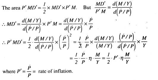
On the other hand, in the Keynesian approach, the cost of inflation is taken as the socially undesirable redistribution of income. In. Fig. 16.11 the cost of inflation can be measured by the area P’MD’ and this area can be approximated by the formula, ½ P’ M/Y n, where P’ is the rate of inflation, M/Y is the ratio of money to income and n is the inflation elasticity of the ratio of money to income.

This can be shown as follows:

This inflation cost or tax represents the welfare loss in order to economise the use of cash balances. This social loss appears from the substitution of real resources for money. The empirical studies seem to confirm that the quantity theory approach is more acceptable in a number of ways over the Keynesian approach. For the mixed type of inflation, however, the quantity theory approach has not proved very useful.

Mark-Up Inflation:

The theory of mark-up inflation assumes that the price of a commodity is determined on the basis of some standard mark-up over the average direct cost of production. The theory of mark-up pricing and inflation has been developed to make the business community as much responsible as the trade unions for an inflationary situation.

According to the mark-up theory of inflation the price of product is determined by the seller in the following way; an estimate is made of the average direct cost of labour and raw materials on the basis of their prices and the expected level of production; then a costing margin is added to the average direct cost to cover the overhead expenses and the expected profit; the costing margin is expressed as a percentage of the average direct cost.

This is also called the percentage mark-up which, when added to the average cost, gives the price per unit. When the market is dominated by oligopolistic firms, price-formation in this way is the general rule. In the labour market, the trade unions are supposed to follow the same procedure to determine their wage rate.

On the basis of the prevailing price level, the average cost is estimated, and, then, a percentage mark-up is added to the average cost of living to determine the wage rate. The percentage mark-up employed by the trade unions for the formation of the wage rate is based on the bargaining strength of the Unions and their expectation of a share in the improvement of productivity in the economy.

Under mark-up pricing theory the cost-push tends to be facilitated for the following reasons. First, the price rise follows directly and, thus, more rapidly upon the wage increases. Second, when prices are not sensitive to demand, profit rates tend to be maintained. The resulting price is fixed at a higher level than short-run profit maximisation. Third, management will put up less resistance to wage claims when mark-up pricing is used.

The mark-up inflation is generalized as income inflation. The basic idea of income inflation is that, at full employment, different groups of people in the economy attempt to improve or maintain their real income by raising their money incomes. If output cannot be increased to satisfy expectations, prices must rise and all groups of people in the economy experience some frustration. The process may continue so long as these frustrated groups try to improve their economic position to suit their monetary objectives.

The process will stop when all groups adapt to the new monetary arrangements. This process is shown in Fig. 16.12 below. In this diagram money income is measured on the vertical axis and the price level on the horizontal axis. All combinations of price level and money income lie on the straight line OO’ and represents the same real income. Let OB represent the fixed money claims of the rentier group.

Let π and W curves represent the claims of profit and wage recipients, respectively. Let π + W + F represent total claims (C) which exceeds the total real income available at (Y₁ P₁). This leads to a price rise. These conflicting claims are ultimately resolved by the rise in the price at (Y₂, P₂) where the π + w + F curve intersects the OO’ line. At this point, prices cease to rise. This stable equilibrium will not be possible if the W + π + F curve does not intersect the OO’ line at all.

Ackley’s mark-up model of inflation is an adaptation of the theory of income inflation. In this mark-up inflation model, Ackley assumes that all business firms set their prices on some mark-up over the material and labour cost, and the labour seeks an increase in money wages that involves some mark- up over the increase in the cost of living.

Ackley is of the opinion that inflationary process develops in inter firm transactions which also includes a mark-up price. Ackley’s model adds to the income inflation picture in that it relates the price setting process to actual business practice and also that it stresses the insensitivity to demand in the short-run and of administrated wages and prices.

Thus, if all wages and prices were set up by mark-up, an inflation could not be originated from excess demand in the short-run, nor be controlled by deficient demand. However, over the long-run, the situation could be different. Eventually, excess demand may induce an increase in the rates of mark-up and, thus, beginning or accelerating an inflation without a cost increase.

As there is always a competitive sector in the agricultural commodities and other inputs, excess demand may induce a mark-up inflation via rises in the prices of inputs. The mark-up inflation points out that labour is not solely responsible for cost inflation. It is a combination of wage claims and business pricing policies that may be responsible for producing inflation.

Anti-Inflation Policies:

Anti-inflation policies may be grouped as:

(1) Monetary Policy

(2) Fiscal Policy and

(3) Non-Monetary Policy.

Let us discuss these policies one by one.

(1) Monetary Policy:

The monetary policy refers to the Credit Control Policy of the central bank.

The central bank can take the following measures to control the volume of credit:

(a) Open Market Operations:

means that, government can reduce or eliminate the excess purchasing power by selling government securities in the open market. This will reduce the purchasing power of the public as they are buying government securities rather than commodities. This would reduce the quantity of money in the economy,

(b) Changes in the Bank Rate:

The bank rate should be increased during a period of inflation. The increase in the bank rate will increase the long-‘ run market rate of interest, thereby discouraging investment. This will reduce the inflationary gap.

(c) Changes in the reserve ratio to be maintained by the Commercial Banks with the central bank. The reserve ratio of the Commercial Banks will have to be increased during the period of inflation. When the reserve ratio is raised, this will reduce the excess reserves of the commercial banks and thus, reduce the credit creating capacity of the banking system and

(d) Selective methods of credit control :

To control credit in some selective sectors of the economy the selective methods of credit control like regulation of margin requirements or regulation of consumer credit may be used. The main difficulty with the monetary policy is that, it works only indirectly. Hence, the result to be obtained by adopting monetary policy would require some time lag. Moreover, the extent to which the monetary policy will be successful depends on the sensitivity of different economic variables to changes in the supply of money and the rate of interest.

(2) Fiscal Policy:

As a result, of these difficulties with the monetary policy, fiscal policy may also be used to control inflation. The fiscal policy refers to taxation and expenditure policies of the government. Different fiscal parameters, such as the changes in the government expenditure including transfer payments, changes in taxes or changes in government borrowing, can directly affect aggregate demand.

During the period of inflation it can take the following steps:

(a) Government can reduce its expenditure which will reduce aggregate demand as government expenditure is a component of aggregate demand.

(b) Taxes should be increased, government expenditure remaining the same. An increase in taxes will reduce the disposable income and, thereby, reducing consumption expenditure. It should be noted that, as anti-inflationary measures, direct taxes are superior to indirect taxes. Since the impact of indirect taxes can be shifted, imposition of indirect taxes will lead to an increase in the price level.

(c) The government should borrow from the public during a period of inflation by selling bonds. When people buy bonds, they surrender purchasing power, which may, otherwise, have been spent on consumption or investment.

(3) Non-Monetary Policy:

Apart from the monetary and Fiscal measures, non-monetary policies may also be adopted to control inflationary situation. The most commonly used anti-inflationary measure, other than restricting demand, has been income policies.

It refers to a wide range of policies running from the government’s setting of voluntary guidelines for wages and price increases, through consultation on wage and price norm between unions, management and government to compulsory controls on wage, price and profit increases. These are basically interventionist policies that call for government action to alter the results, that would otherwise have emerged from private- sector bargaining.

Income policies have been used in Europe in all sorts of circumstances. The non-monetary measures may also include output adjustments and rationing, etc. Inflation may arise because of shortage of output. Thus, to control inflation, the level of output should be increased in real terms. The measures to control price and rationing are actually short-run measures. Price control means fixation of legal upper limit for prices of goods.

However, if demand cannot be controlled, mere price control may lead to the creation of black market. Rationing functions as a device of stabilising consumer prices and assuring distributive justice. However, rationing by weak administration may lead to black market and corruption. Different anti-inflationary policies should not be regarded as competitive. They are rather complementary. All of them should be used together to get the best result.