Measuring the Substitution Effect: Top 2 Methods (With Diagram)

The following points highlight the top two methods of measuring the substitution effect. The methods are: 1. Hicks’ Substitution Effect 2. Slutsky’s Substitution Effect.

Method # 1. Hicks’ Substitution Effect:

Prof. Hicks has explained the substitution effect independent of the income effect through compensating variation in income.

“The substitution effect is the increase in the quantity bought as the price of the commodity falls, after adjusting income so as to keep the real purchasing power of the consumer the same as before. This adjustment in income is called compensating variations and is shown graphically by a parallel shift of the new budget line until it become tangent to the initial indifference curve.”

Thus on the basis of the methods of compensating variation, the substitution effect measure the effect of change in the relative price of a good with real income constant. The increase in the real income of the consumer as a result of fall in the price of, say good X, is so withdrawn that he is neither better off nor worse off than before.

The substitution effect is explained in Figure 28 where the original budget line is PQ with equilibrium at point R on the indifference curve I₁,. At R, the consumer is buying OB of X and BR of Y. Suppose the price of X falls so that his new budget line is PQ₁ .With the fall in the price of X, the real income of the consumer increases.

To make the compensating variation in income or to keep the consumer’s real income constant, take away the increase in his income equal to PM of good Y or Q₁N of good X so that his budget line PQ, shifts to the left as MN and is parallel to it.

At the same time, MN is tangent to the original indifference curve I_1; but at point H where the consumer buys OD of X and DH of Y.Thus PM of Y or Q₁N of X represents the compensating variation in income, as shown by the line MN being tangent to the curve I₁ at point H.

Now the consumer substitutes X for Y and moves from point R to H or the horizontal distance from В to D). This movement is called the substitution effect. The substitution affect is always negative because when the price of a good falls (or rises), more (or less) of it would be purchased, the real income of the consumer and price of the other good remaining constant.

In other words, the relation between price and quantity demanded being inverse, the substitution effect is negative.

Method # 2. Slutsky’s Substitution Effect:

Slutsky explained the substitution effect by taking the apparent real income of the consumers constant. With the fall in the price of, say, good X when the real income of the consumer increases, it is adjusted in such a way that the consumer could purchase the same bundle of the two goods as before the price change if he liked, so that his real income remains constant.

But when he moves to a higher indifference curve, the substitution effect takes place.

Prof Hicks call’s Slutsky’s method of measuring the substitution effect as the cost difference method. In the Slutsky substitution effect, the constant real income means constant purchasing power in terms of the particular bundle of two goods.

The cost difference refers to the difference in purchasing power due to a difference in prices. It is calculated by the difference in the cost of a specific bundle of two goods at the old and the new price.

The Slutsky substitution effect is presented in Figure 29 where the original budget line PQ is tangent to the indifference curve I₁ at point R. At this point, the consumer purchases OA of X and AR of Y. Suppose the price of X falls and his new budget line is PQ₁. The fall in the price of X increases the purchasing power or real income of the consumer.

This increased income should be taken away through cost difference in such a manner that the consumer is able to buy the original bundle R of X and Y so that his apparent real income remains constant. For this, the line M₁ N₁ is drawn in such a manner that it passes through point R and is parallel to the line PQ₁.

This is equivalent to reducing the consumer’s income by PM₁ of Y or Q₁N₁ of X. Now the consumer faces the new relative price with constant purchasing power on the price-income line M₁N₁. The consumer cannot be at the original point R on this line because it is not tangent to the I₁ curve at this point.

Instead, he will move to point S on a higher indifference curve I₂ where the price income line M₁N₁ is tangent to it. Since the two lines PQ and M₁, N₁ have the same purchasing power, the difference between their equilibrium positions R and S is due To the substitution effect of the price difference.

Thus the increase in the quantity of X as represented by the movement from point A to С on the horizontal axis is the Slutsky substitution effect due to the fall in the price of X.

Conclusion:

Of the two methods of measuring the substitution effect, Slutsky’s method is superior to Hicks’ method. The Hicksian substitution effect keeps the real income of the consumer constant by bringing him back to the initial level of satisfaction on the original indifference curve.

On the other hand, the Slutsky substitution effect provides the consumer greater satisfaction by bringing him on a higher indifference curve. In the Slutsky method, real income can be calculated equal to cost difference by observing market prices and quantities, whereas Hicks’ compensating variation in income is difficult to estimate.

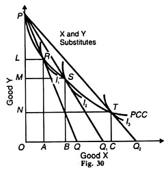
The price effect indicates the way the consumer’s purchases of good X change, when its price changes, given his income, tastes and preferences and the price of good This is shown in Figure 30 Suppose the price of X falls. The budget line PQ will extend further out to the right as P Q, showing that the consumer will buy more of X than before, as X has become cheaper.

The budget line PQ, shows a further fall in the price of X. Each of the budget line fanning out form P is a tangent to an indifference curve I₁, I₂ and I₃ at R, S and T respectively. The curve PCC connecting the locus of these equilibrium points is called the price consumption curve.

The price – consumption curve indicates the price effect of a change in the price of X on the consumer’s purchases of the two goods X and Y, given his income, tastes, preferences and the price of good Y.

In Figure 30 the PCC curve slopes downward. As the price of X falls, the consumer buys more of X and less of Y. Thus at point S on the PCC, he purchases OB of X and OM of Y instead of OA of X and OL of Y at Point R. A downward sloping price-consumption curve thus shows that the two goods X and Y are substitutes for one another.

The cross elasticity of demand between X and Y when they are substitutes is positive. If the PCC curve is horizontal, the cross-elasticity of demand between X and Y is zero which means that X and Y are unrelated goods.

A fall in the price of X though increasing the purchases of good X from OA to В and to С has no effect on the demand for good Y which remains the same as before RA = SB = TC, as shown in Figure 31 (A). If the PCC slopes upward, X and Y are complementary goods. The consumer purchases larger quantities of both the goods at point R, S and T respectively as in Panel (B).

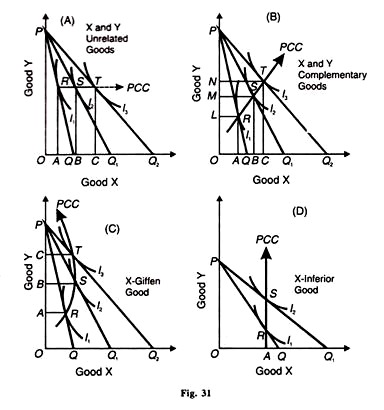
When the price-consumption curve is backward sloping toward the Y-axis as in Panel (C), the cross­ elasticity of demand between X and Y is negative. The demand for X declines from BS to CT with fall in its price from PQ, to PQ₂ and the demand for Y rises from OB to ОС.

X is a Gif fen good in this case, when it becomes cheaper the consumer purchases less of it. Panel (D) shows a vertical PCC signifying that X is an inferior good. A fall in its price from PQ to PQ_: does not lead to rise in its demand which remains constant at OA.