The Harrod-Domar Economic Growth Model (With Assumptions)

Let us make an in-depth study of the Harrod-Domar Economic Growth Model:- 1. Introduction to the Harrod-Domar Economic Growth Model 2. General Assumptions 3. Instability of Growth 4. The Domar Model 5. Summary of Main Points 6. Diagrammatic Representation.

Introduction to the Harrod-Domar Economic Growth Model:

Ever since the end of Second World War, interest in the problems of economic growth has led economists to formulate growth models of different types.

These models deal with and lay emphasis on the various aspects of growth of the developed economies. They constitute in a way alternative stylized pictures of an expanding economy.

A feature common to them all is that they are based on the Keynesian saving-investment analysis. The first and the simplest model of growth—the Harrod-Domar Model—is the direct outcome of projection of the short-run Keynesian analysis into the long-run.

This model is based on the capital factor as the crucial factor of economic growth. It concentrates on the possibility of steady growth through adjustment of supply of demand for capital. Then there is Mrs. Joan Robinson’s model which considers technical progress also, along with capital formation, as a source of economic growth. The third type of growth model is that built on neo­classical lines.

It assumes substitution between capital and labour and a neutral technical progress in the sense that technical progress is neither saving nor absorbing of labour or capital. Both the factors are used in the same proportion even when neutral technical takes place. We deal with the prominent growth models here.

Although Harrod and Domar models differ in details, they are similar in substance. One may call Harrod’s model as the English version of Domar’s model. Both these models stress the essential conditions of achieving and maintaining steady growth. Harrod and Domar assign a crucial role to capital accumulation in the process of growth. In fact, they emphasise the dual role of capital accumulation.

On the one hand, new investment generates income (through multiplier effect); on the other hand, it increases productive capacity (through productivity effect) of the economy by expanding its capital stock. It is pertinent to note here that classical economists emphasised the productivity aspect of the investment and took for granted the income aspect. Keynes had given due attention to the problem of income generation but neglected the problem of productive capacity creation. Harrod and Domar took special care to deal with both the problems generated by investment in their models.

General Assumptions:

The main assumptions of the Harrod-Domar models are as follows:

(i) A full-employment level of income already exists.

(ii) There is no government interference in the functioning of the economy.

(iii) The model is based on the assumption of “closed economy.” In other words, government restrictions on trade and the complications caused by international trade are ruled out.

(iv) There are no lags in adjustment of variables i.e., the economic variables such as savings, investment, income, expenditure adjust themselves completely within the same period of time.

(v) The average propensity to save (APS) and marginal propensity to save (MPS) are equal to each other. APS = MPS or written in symbols,

S/Y= ∆S/∆Y

(vi) Both propensity to save and “capital coefficient” (i.e., capital-output ratio) are given constant. This amounts to assuming that the law of constant returns operates in the economy because of fixity of the capita-output ratio.

(vii) Income, investment, savings are all defined in the net sense, i.e., they are considered over and above the depreciation. Thus, depreciation rates are not included in these variables.

(viii) Saving and investment are equal in ex-ante as well as in ex-post sense i.e., there is accounting as well as functional equality between saving and investment.

These assumptions were meant to simplify the task of growth analysis; these could be relaxed later.

Harrod’s growth model raised three issues:

(i) How can steady growth be achieved for an economy with a fixed (capital- output ratio) (capital-coefficient) and a fixed saving-income ratio?

(ii) How can the steady growth rate be maintained? Or what are the conditions for maintaining steady uninterrupted growth?

(iii) How do the natural factors put a ceiling on the growth rate of the economy?

In order to discuss these issues, Harrod had adopted three different concepts of growth rates: (i) the actual growth rate, G, (ii) the warranted growth rate, G_w (iii) the natural growth rate, G_n.

The Actual Growth Rate is the growth rate determined by the actual rate of savings and investment in the country. In other words, it can be defined as the ratio of change in income (AT) to the total income (Y) in the given period. If actual growth rate is denoted by G, then

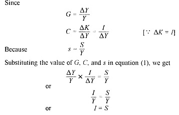
G = ∆Y/Y

The actual growth rate (G) is determined by saving-income ratio and capital- output ratio. Both the factors have been taken as fixed in the given period. The relationship between the actual growth rate and its determinants was expressed as:

GC = s …(1)

where G is the actual rate of growth, C represents the capital-output ratio ∆K/∆Y and s refers to the saving-income ratio ∆S/∆Y. This relation stales the simple truism that saving and investment (in the ex- post sense) are equal in equilibrium. This is clear from the following derivation.

This relation explains that the condition for achieving the steady state growth is that ex-post savings must be equal to ex-post investment. “Warranted growth” refers to that growth rate of the economy when it is working at full capacity. It is also known as Full-capacity growth rate. This growth rate denoted by G_w is interpreted as the rate of income growth required for full utilisation of a growing stock of capital, so that entrepreneurs would be satisfied with the amount of investment actually made.

Warranted growth rate (G_w) is determined by capital-output ratio and saving- income ratio. The relationship between the warranted growth rate and its determinants can be expressed as

G_w C_r = s

where C_r shows the needed C to maintain the warranted growth rate and s is the saving-income ratio.

Let us now discuss the issue: how to achieve steady growth? According to Harrod, the economy can achieve steady growth when

G = G_w and C = C_r

This condition states, firstly, that actual growth rate must be equal to the warranted growth rate. Secondly, the capital-output ratio needed to achieve G must be equal to the required capital-output ratio in order to maintain G_w, given the saving co-efficient (s). This amounts to saying that actual investment must be equal to the expected investment at the given saving rate.

Instability of Growth:

We have stated above that the steady-state growth of the economy requires an equality between G and G_w on the one hand and C and C_r on the other. In a free-enterprise economy, these equilibrium conditions would be satisfied only rarely, if at all. Therefore, Harrod analysed the situations when these conditions are not satisfied.

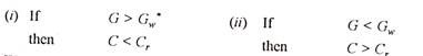
We analyse the situation where G is greater than G_w. Under this situation, the growth rate of income being greater than the growth rate of output, the demand for output (because of the higher level of income) would exceed the supply of output (because of the lower level of output) and the economy would experience inflation. This can be explained in another way too when C < C_r Under this situation, the actual amount of capital falls short of the required amount of capital.

This would lead to deficiency of capital, which would, in turn, adversely affect the volume of goods to be produced. Fall in the level of output would result in scarcity of goods and hence inflation. This, under this situation the economy will find itself in the quagmire of inflation.

On the other hand, when G is less than G_w, the growth rate of income would be less than the growth rate of output. In this situation, there would be excessive goods for sale, but the income would not be sufficient to purchase those goods. In Keynesian terminology, there would be deficiency of demand and consequently the economy would face the problem of deflation. This situation can also be explained when C is greater than C_r.

Here the actual amount of capital would be larger than the required amount of capital for investment. The larger amount of capital available for investment would dampen the marginal efficiency of capital in the long period. Secular decline in the marginal efficiency of capital would lead to chronic depression and unemployment. This is the state of secular stagnation.

From the above analysis, it can be concluded that steady growth implies a balance between G and G_w. In a free-enterprise economy, it is difficult to strike a balance between G and G_w as the two are determined by altogether different sets of factors. Since a slight deviation of G from G_w leads the economy away and further away from the steady-state growth path, it is called ‘knife-edge’ equilibrium.

G_n the Natural growth rate is determined by natural conditions such as labour force, natural resources, capital equipment, technical knowledge etc. These factors place a limit beyond which expansion of output is not feasible. This limit is called Full-Employment Ceiling. This upper limit may change as the production factors grow, or as technological progress takes place. Thus, the natural growth rate is the maximum growth rate which an economy can achieve with its available natural resources. The third fundamental relation in Harrod’s model showing the determinants of natural growth rate is

G_nC_r is either = or ≠s

Interaction of G, G_w and G_n:

Comparing the second and the third relations about the warranted growth rate and the natural growth rate which have been given above, we may conclude that G_n may or may not be equal to G_w. In case G„ happens to be equal to G_w, the conditions of steady growth with full employment would be satisfied. But such a possibility is remote because of the variety of hindrances are likely to intervene and make the balance among all these factors difficult. As such there is a definite possibility of inequality between G_n and G_w. If G„ exceeds G_w, G would also exceed G_w for most of the time as is shown in Figure 17.1, and there would be a tendency in the economy for cumulative boom and full employment.

Such a situation will create an inflationary trend. To check this trend, savings become desirable because these would enable the economy to have a high level of employment without inflationary pressures. If on the other hand G_w exceeds G„, G must be below G„ for most of the time and there would be a tendency for cumulative recession resulting in unemployment (Figure 17.2).

The Domar Model:

The main growth model of Domar bears a certain resemblance to the model of Harrod. In fact, Harrod regarded Domar’s formulation as a rediscovery of his own version after a gap of seven years.

Domar’s theory was just an extension of Keynes’ General Theory, particularly on two counts:

1. Investment has two effects:

(a) An income-generating effect and

(b) Productivity effect by creating capacity.

The short-run analysis governed by Keynes ignored the second effect.

2. Unemployment of labour generally attracts attention and one feels sympathy for the jobless, but unemployment of capital attracts little attention. It should be understood that unemployment of capital inhibits investment and hence reduces income. Reduction of income brings about deficiency in demand and hence unemployment. Thus the Keynesian concept of unemployment misses the root cause of the problem. Domar wanted to analyse the genesis of unemployment in a wider sense.

To understand the implications of Domar model, one should get familiar with the relations listed below:

1. Income is determined by investment through multiplier. For simplicity saving-income ratio (s) is assumed constant. This implies that

Y_(t) = I_(t)/s

where Y is the output, I is the actual investment and s is saving-income ratio (saving propensity) and (t) shows the time period.

2. Productive capacity is created by investment to the extent of the potential (social) average productivity of investment denoted by a. For simplicity, this is also assumed to be constant. In notation form the relation can be written as

Y_(t) –Y_(t-1)= I_(t)/α

where Y shows the productive capacity for output, a is the actual marginal capital-output ratio which is the reciprocal of “potential social average investment productivity” (α= 1/σ). Therefore, Equation (2) can also be expressed as ∆Y_t = σI_t. This equation shows that the change in productive capacity is the product of capital productivity (σ) and investment. As such it reveals the productivity effect.

3. Investment is induced by output growth along with entrepreneurial confidence. The latter is adversely affected by “Junking” which means the untimely loss of capital value due to the unprofitable operation of older facilities. This may be due to the shortage of labour or invention of new products or labour-saving inventions. This assumption can be shown by the relation

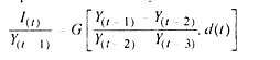
where G is an increasing function of the rate of output acceleration, but a decreasing function of the “Junking ratio” d(t).

If junking ratio is zero then investment increases at the same rate as output

4. Employment depends upon the ‘utilization ratio’ expressed as the ratio between actual output and productive capacity. It may be expressed as

Here A’ refers to employment and L to the labour force. II is the employment coefficient, Y^d the actual output and the productive capacity, (I) being the time period. This equation explains that the ratio of employment to labour force is determined by employment coefficient (II) and the ratio of output to productivity. The dots are meant to indicate the existence of other determinants of the employment ratio. If we assume that the employment coefficient takes the maximum value of unity (i.e., H = I), then Yd_(t) = Y^s_(t)

5. Past as well as present investment can generate productive capacity at a given ratio. But due to managerial miscalculation, the new investment projects will cause untimely demise of old project and plants. If “junking” exists, it would dampen the productivity of investment. This assumption is considered the central theme of Doinar’s model. In the form of notations, it can be expressed as

where K is capital, / shows investment, d(t). K(t) is the amount of capital junked, and d(t) is the junking ratio.

Domar viewed growth from the demand as well as the supply side. Investment on the one side increases productive capacity and on the other generates income. Balancing of the two sides provides the solution for steady growth. The following symbols are used in Domar’s model.

Y_d = level of net national income or level of effective demand at full employment (demand side)

Y_s = level of productive capacity or supply at full-employment level (supply side)

K = real capital

I = net investment which results in the increase of real capital i.e., ∆K a = marginal propensity to save, which is the reciprocal of multiplier. a = (sigma) is productivity of capital or of net investment.

The demand side of the long-term effect of investment can be summarised through the following relation. This relation is a simple application of Keynes investment multiplier.

Y_d = 1/a . I

This relation tells us (I) that the level of effective demand (Y_d) is directly related to the level of investment through the multiplier whose value is given by 1/α. Any increase in the level of investment will directly increase the level of effective demand and vice versa. (ii) The effective demand is inversely related to the marginal propensity to save (a). Any increase in marginal propensity to save (a) will decrease the level of effective demand and vice versa.

The supply side of the economy in the Domar model is shown through the relation.

Y_s = σK

This relation explains that the supply of output (Y_s) at full employment depends upon two factors: productive capacity of capital (σ) and the amount of real capital (K). Any increase or decrease in one of these two factors will change the supply of output. If the productivity of capital (σ) increases, that would favorably affect the economy’s supply. Similar is the effect of the change in the real capital K on the supply of output.

For the economy’s long-term equilibrium, the demand Y_d and supply Y_s sides should be equal. Therefore, we can write:

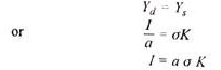
This relation tells us that steady growth is possible when investment over a period of time equals the product of saving-income ratio, capital productivity and capital stock.

The demand and the supply equation in the incremental form can be written as follows: The demand side is:

∆Y_d =∆I/α …(1)

But the increment has not been shown in a because it is a constant in terms of the assumptions. Since 1/α is nothing but a and ∆I leads to ∆K, we can write the supply relation as follows:

∆Y_s = σ ∆K

This equation shows that a change in the supply of output (∆Y_s) can be expressed as the product of the change in real capital (∆K), and the productivity of capital (σ). Substituting the value of ∆K as I in the above equation, we get the supply side of the economy as

∆Y_s= σ I …(1)

From equations (1) and (2) we can derive the condition for steady growth. Using equations (1) and (2), we get

Equation (3) explains that if steady growth is to be maintained, the income growth rate ∆Y/Y should be equal to the product of marginal propensity to save (α) and the productivity of capital (α). In the words of K.K. Kurihara “It is an increase in productive capacity (∆Y_s) due to increment of real capital (∆C) which must be matched by an equal increase in effective demand (∆Y_d) due to an increment of investment (∆I), if a growing economy with an expanding stock of capital is to maintain continuous full-employment.

Domar’s condition of steady state growth can be explained with the help of numerical example. Suppose the productivity of capital (σ) is 25% and the marginal propensity to save is 12%, then the growth rate of investment (AHI) would be equal to a, a, i.e.,

Thus income and investment must grow at the annual rate of 3% if steady growth rate is to be maintained.

Analysis of disequilibrium:

Disequilibrium (non-steady state) prevails

Under the first situation, long-term inflation would appear in the economy because the higher growth rate of income will provide greater purchasing power to the people and the productive capacity (σα) would not be able to cope with the increased level of income. The first situation of disequilibrium will, therefore, create inflation in the economy.

The second situation, under which growth rate of income or investment is lagging behind the productive capacity, will result in over production. The reduced growth rate of income will put a constraint on the purchasing power of the people, thereby reducing the level of demand and resulting in over-production. This is the situation in which there would be secular stagnation. We have thus arrived at the same conclusion of instability of stendy growth which we had derived from the Harrod model.

Summary of Main Points:

The main points of the Harrod-Domar analysis are summarised below:

1. Investment is the central variable of stable growth and it plays a double role; on the one hand, it generates income and on the other, it creates productive capacity.

2. The increased capacity arising from investment can result in greater output or greater unemployment depending on the behaviour of income

3. Conditions concerning the behaviour of income can be expressed in terms of growth rates i.e. G, G_w and G_n and equality between the three growth rates can ensure full employment of labour and full-utilisation of capital stock.

4. These conditions, however, specify only a steady-state growth. The actual growth rate may differ from the warranted growth rate. If the actual growth rate is greater than the warranted rate of growth, the economy will experience cumulative inflation. If the actual growth rate is less than the warranted growth rate, the economy will slide towards cumulative inflation. If the actual growth rate is less than the warranted growth rate, the economy will slide towards cumulative deflation.

5. Business cycles are viewed as deviations from the path of steady growth. These deviations cannot go on working indefinitely. These are constrained by upper and lower limits, the ‘full employment ceiling’ acts as an upper limit and effective demand composed of autonomous investment and consumption acts as the lower limit. The actual growth rate fluctuates between these two limits.

Diagrammatic Representation:

Refer to Figure 17.3 where income is shown on the horizontal axis, Saving and Investment on ver­tical axis. The line S(Y) drawn through the origin shows the levels of saving corresponding to different levels of income. The slope of this line (tangent α) measures the aver­age and marginal propensity to save. The slopes of lines Y₀I₀, Y₁I₁, Y₂I₂ measure the acceleration co-efficient v which remains constant at each income level of Y₀, Y₁, and Y₂.

At the initial income level of Y₀, the saving is S₀Y₀. When this saving is invested, income rises from Y₀ to Y₁. This higher level of income in­creases saving to S₁Y₁. When this amount of saving is reinvested, it will further raise the level of income to Y₂. The higher level of income will again raise saving to S₂Y₂. This process of rise in income, saving and investment shows the accelera­tion effect on the growth of output.

Now we give the diagram­matic exposition of the Harrod model with the help of Figure 17.4.

In this figure, income is shown on horizontal axis, saving and investment on vertical axis. The line S(Y) passing through the origin indicates the level of saving corresponding to different levels of income. I₀I₀, I₁I₁ and I₂I₂ are the various levels of investment. Y₀P₀ and Y₁P₁ measure the productivity of capital corresponding to different levels of investment.

The lines Y₀P₀ and Y₁P₁ are drawn parallel so as to show that productivity of capital remains unchanged. This diagram shows that the level of income is determined by the forces of saving and investment. The level of income Y₀ is determined by the intersection of saving line S(Y) and the investment line I₀I₀.

At the level of income Y₀, the saving is Y₀S₀. When the saving Y₀S₀ is invested, it will increase the income level from OY₀ to OY₁. The productive capacity will also rise correspondingly. The extent of the income increase depends upon the productivity of capital, which is measured by the slope of the line Y₀P₀ (α).

Higher is the level of income higher the productive capacity. Similarly, when the level of income is OY₁ the level of saving is S₁Y₁. With investment of S₁Y₁ income will further rise to the level Y₂. This increase in income means expansion of purchasing power of the economy. But the coefficient of capital productivity would remain constant, this being an important assumption of Domar’s model.