A function describes the relation between two or more than two variables.
That is, a function expresses dependence of one variable on one or more other variables.
Thus, if the value of a variable V depends on another variable X, we may write:
Y=f (X) …. (1)
ADVERTISEMENTS:
Where f stands for function.
This expression (1) is read as ‘Y is function of X’. This implies that every value of the variable Y is determined by a unique value of the variable X. In the function (1) Y is known as the dependent variable and X is the independent variable. Thus in function (1) Y is called the dependent variable and its value depends on the value of X Further, the independent variable is Interpreted as the cause and the dependent variable as the effect. An important function which is extensively used in economics is a demand function which expresses quantity demanded of a commodity is a function of its price, other factors being held constant.
Thus, demand for a commodity X is described as under:
Dx =f (Px)
ADVERTISEMENTS:
Where Dx is the quantity demanded of commodity X and Px is its price.
Similarly, supply function of a commodity X is expressed as:
Sx = f (Px)
When the value of the variable Y depends on more than two variables X1, X2….. Xn this function is written in general form as:
ADVERTISEMENTS:
Y = f (X1, X2, X3, X4………. Xn)
This shows the variable Y depends on several independent variables X1, X2……Xn where n is the number of independent variables. Again note that in economics we write ’causes’ as the independent variables and ‘effect’ as the dependent variable.
For example, demand for a product is generally considered to be a function of its own price prices of other commodities (which may be substitutes or complements) income of the consumers, tastes and preferences of the consumers and advertising expenditure made by a firm to promote its product. Thus,
Dx = f (Px, PY, M, T, A)
Where
Dx = demand for the commodity X
Px = price of the commodity X
Py = price of a substitute product
M= income of the consumers
ADVERTISEMENTS:
T = tastes and preferences of the consumer for the product.
A = advertising expenditure incurred by the firm.
The exact nature of relation of dependent variable with the independent variables can be known from the specific form of the function. The specific form of a unction can take a variety of mathematical forms. We explain below some specific types of functions.
Linear and Power Functions:
A widely used mathematical form of a function is a linear function.
ADVERTISEMENTS:
A linear function can be stated in the following general form:
Y = a + bX
Where a and b are positive constants and are called parameters of the function. Note that parameters of a function are variables that are fixed and given in a specific function. The values of constants a and b determine the specific nature of a linear function.
The linear demand function with price as the only independent variable is written as:
ADVERTISEMENTS:
Qd = a – bP
The minus sign before coefficient b indicates that quantity demanded of a commodity is negatively related with price of the commodity. That is, if price of a commodity falls, its quantity demand increases and vice versa.
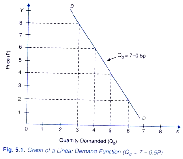
If a equals 7 and b equals 0.5, the linear demand function can be expressed in the following specific form:
Qd = 7 – 0.5 P
The above specific demand function shows that a unit fall in price of the commodity will cause 0.5 units increase in the quantity demanded of the commodity. If price (P) is zero, the second term (0.5P) in the demand function drops out and the quantity demanded is equal to 7.
We can take various values of P and find out different quantities (Qd) of a commodity demanded at them. In Figure 5.1 we have noted these price-quantity combinations on a graph and have obtained demand curve DD of the commodity representing the given demand function (Qd = 7- 0.5P).
ADVERTISEMENTS:
It should be noted that, contrary to mathematical practice, by convention in economics to represent demand function we show the independent variable (price in the above case of demand function) on the y-axis and the dependent variable (the quantity demanded in the present case) on the x-axis. Graph of linear demand function is shown in Figure 5.1.
It is worth noting that slope of the demand function curve in Figure 5.1 will represent ∆P/ ∆Q. However, if we represent quantity demanded (Qd) on the y-axis, and price (Px) on the x-axis; the slope of the demand curve so drawn would be equal to ∆Q/∆P.
Multivariate Linear Demand Function:
Linear demand function with more than one independent variables, can be written in the following way:
Qx = a + b1 Px + b2 Py+ b3 M + b4 T + b5 A
Where b1, b2, b3, b4, are the coefficients of the respective variables. In economics the effect of variables other than the own price of a commodity in the demand function are depicted by shifts in the demand curve. For instance when income (M) of the consumers increases consumers will demand more of the product X at a given price. This implies shifting of the demand curve to the right.
ADVERTISEMENTS:
The linear multivariate function is written in the following form:
Y = 4 – o.4X1 + 0.2X2+ 0.3X3 + 0.5 X4
In this function the coefficients 0.4, 0.2, 0.3 and 0.5 show the precise impact of the independent variables X1, X2, X3, X4 on the dependent variable Y.
Power Functions:
The linear functions stated above are known as first degree functions where the independent variables X1, X2, X3, etc. are raised to the first power only. We now turn to explain power functions. In economics power functions of the quadratic and cubic forms are extensively used.
Quadratic Functions:
In quadratic function one or more of the independent variables are squared, that is, raised to the second power. Note that power is also referred to as exponent A quadratic function may be written as
Y = a + b X+ c X2
ADVERTISEMENTS:
This implies that value of the dependent variable Y depends on the constant a plus the coefficient b times the value of the independent variable X plus the coefficient c times the square of the variable X Suppose a = 4, b = 3 and c = 2 then quadratic function takes the following specific form.
Y = 4 + 3X+2 X2
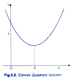
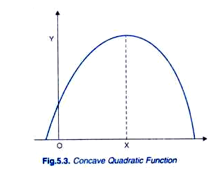
We can obtain the different values of Y for taking different values of the independent variable X. Quadratic functions are of two types: convex quadratic functions and concave quadratic functions. The form of quadratic function depends on the sign of the coefficient c of X2. The quadratic function, Y = a + bX + cX2, where the coefficient c of X2 is positive (i.e. c > 0) is called convex quadratic function, because its graph is U-shaped as shown in Figure 5.2. On the other hand, if coefficient of X2 is negative (c < 0), that is, when Y= a + bX- cX2 then we have concave quadratic function because its graphs is of inverted ᴒ- shape (i.e. n-shaped) as shown in Figure 5.3.
It is worth noting that slope of the curve of convex quadratic functions as is evident from U-shaped graph in this case where coefficient of X2 is positive, slope is increasing everywhere. On the other hand, in case of concave quadratic function where coefficient of is negative (c < 0), slope of its graph is decreasing everywhere. It should be further noted that in analytical geometry it is proved that graph of any quadratic function is a parabola which may be either convex or concave. A parabola is a curve which has a turning point and unlike the curve of a linear function, its slope is changing at different values of X.
Multivariable Quadratic Function:
ADVERTISEMENTS:
When there are more than one independent variable such as X1, X2, and they have a quadratic relationship with the dependent variable Y, such a function is called multivariable quadratic function.
In case of two independent variables X1 and X2 such a function may be expressed as under:
Y = a + bX1 – cX21 + dX2– eX22
If such a function is graphically shown, it will be represented by a three dimensional surface and not a two dimensional curve.
Cubic Function:
A cubic function is the power function in which there is a third degree term relating to an independent variable. Thus, a cubic functions may have first degree, second degree and third degree terms.
A cubic function may have the following form:
Y = a+ bX+cX2 + dX3
a is the intercept term, the dependent variable X has the first degree, second degree and third degree terms. When the signs of all the coefficients a, b, c and d are positive, then the values of y will increase by progressively larger increments as the value of X increases. However, when the signs of various coefficients differ in the cubic function, that is, some have positive signs and some have negative signs, then the graph of the function may have both convex and concave segments depending on the values of the coefficients.
Such a cubic function where signs of the coefficients of variables differ may be expressed as follows:
Y = a + bX-cX2 + dX3
In which the sign of the coefficient c of variable X^ is negative whereas the coefficients of others are positive.
Slopes of Functions:
In economics it is important to know the rate at which a variable changes in response to a change in another variable, the slope of a variable measures this rate. For example, it is important to know the rate at which quantity demanded of a commodity changes in response to a change in price of a commodity. In the field of economics we find both linear and nonlinear functions. Let us first take the slope of a linear function.
Consider the following linear function:
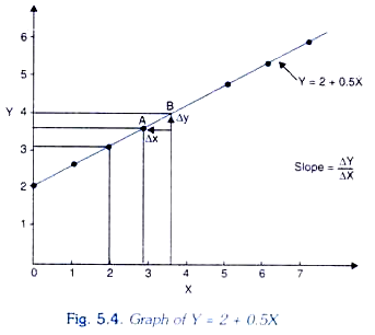
Y = f (X) = 2 + 0.5 X
In Table 5.1 we have calculated the values of the variable Y by taking different values of X such as 1, 2, 3, 4 etc. Further, we have plotted the different values of Table 5.1 on a graph shown in Fig. 5.4. The slope of the function, (Y = 2 + 0.5X) between two points, say, A and B in Figure 5.4 is given by the ratio of change in Y to the change in X. That is, slope = ∆Y / ∆X.
For example, at point A of the given function value of variable X is 3 and corresponding to it the value of variable Vis 3.5. When value of X rises from 3 to 4, value of Y increases from 3.5 to 4.
Thus, the slope of the function (Y=2 + 0.5X) is:
∆Y/ ∆X = 4-3.5/ 0.5 = 0.5 / 1 = 0.5
This implies that value of Y increases by 0.5 when value of X increases by 1. It should be noted that slope of a linear function is constant throughout.
However, the slope of a linear function can be directly known from the linear function itself and for that purpose there is no need to plot the data. Consider the following linear function
Y = a + bX
It will be seen from this linear function that when the value of X is zero, the value of Y will be equal to a. Thus a is Y intercept. Further, in this function b is the coefficient of X and measures change in Y due to change in X that is, ∆Y/∆X. Thus, b represents the slope of the linear function. In linear function Y= 2 + 0.5X, 2 is the Y-intercept, that is, value of Y when X is zero, 0.5 is the b coefficient which measures the slope of the linear function.
Slope of a Non-linear Function:
We now turn to explain how slope of a non-linear function, say, a quadratic function (Y= a + bX+ cX2) can be measured. On plotting the non-linear function in a graph, we get a non-linear curve.
Let us take the following specific quadratic function:
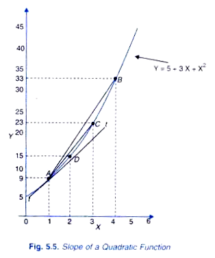
Y = 5 + 3X+X2
In Table 5.2 we have calculated the various values of Y by taking different values of X (0, 1, 2, 3, etc.)
The data so obtained have been plotted to get a curve in Figure 5.5. It will be seen from this Figure 5.5 that slope of the line AB which connects two points A and B on a curve representing quadratic function can be measured by taking the change in the value of Y divided by the change in value of X. At point A, value of X is 1 and the corresponding value of Y is 9 and at point B, the value of X is 4 to which the corresponding value is 33. Thus, here ∆X = 4 – 1 = 3 and ∆y = 33 – 9 = 24.
Thus, the slope of the line AB is:
∆Y/ ∆X =24/3 =8
Similarly, slope of straight line AC in Fig.5.5. can be measured. Between two points A and C, ∆X = 3 – 1 = 2 and ∆Y = 23 – 9 = 14, Thus, the slope of straight line AC is
∆Y/ ∆X = 14/2 =7
In a similar fashion, the slope of the straight line AD connecting points A and D on the non-linear quadratic function curve in Figure 5.5 is given by
∆Y/ ∆X = 15-9/2-1 = 6/1 = 6
It will thus be seen that as AX decreases; it was 3 between A and B, 2 between and C and 1 between A and D, slope of the non-linear curve goes on declining. It was 8 of the line AB 7 of the line AC and 6 of the line AD. As AX further decreases, slope of the line connecting two points of the non-linear curve will further decline.
It should also be noticed that the slope of the straight line AD connecting points and D is very close to the slope of the tangent drawn to the curve at point As AX becomes smaller and smaller slope of the line connecting the two points on a curve will become extremely close to the slope of the tangent drawn to the curve at point A. Therefore, the slope at a point on the non-linear function curve can be measured by the slope of a tangent drawn to the curve at that point.
