The process of optimisation often requires us to determine the maximum or minimum value of a function.
For a function to be a maximum (or minimum) its first derivative is zero. Derivative of a function measures its slope.
Therefore, maximization of a function occurs where its derivative is equal to zero. Thus, an important optimisation problem facing a business manager is to produce a level of output which maximises firm’s profits. Similarly, optimum use of resources requires that cost be minimised for producing a given level of output. These problems of maximisation and minimisation can be solved with the use of the concept of derivative.
1. Use in Profit Maximisation:
For example, consider the following profit function:
ADVERTISEMENTS:
π = -100+ 160Q-10Q2
Where π = profits and Q is units of output
For the profit (π) function to be maximum, its first derivative must be equal to zero.
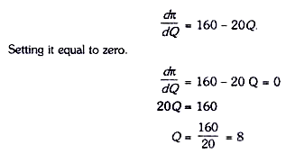
Therefore, to find the profit-maximising level of output we find the derivative of the given profit functions and set it equal to zero. Thus
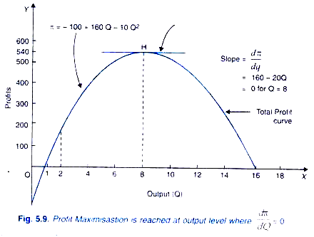
At 8 units of output profits will be maximum. Maximisation of profits through the use of derivative is graphically shown in Figure 5.9. It will be seen that profit maximisation curve reaches its maximum point at point H. Therefore, at point H, the slope of the tangent (which measures the value of derivative dπ / dQ) drawn to the profit curve at this point is equal to zero.
It will be seen that corresponding to maximum profit point H on the profit function level of output is 8 units.
Total profits made at 8 units of output can be obtained by substituting 8 for Q in the given profit function. Thus
π = – 100 + 160 x 8 – 10 (8)2
ADVERTISEMENTS:
= 1280 – 740 = 540
Thus at output level of 8 units profits are equal to 540.
Graphical analysis cannot tell us easily exactly at what level of output, profits will be maximum, for it takes time to draw a graph and conclude from it. However, it is easier to use differential calculus to find the profit-maximising output. For this we simply find the first derivative of the profit function and set it equal to zero.
2. Second Derivative and Second Order Condition for Optimisation:
A problem arises when we use the first derivative of a function to determine its maximum or minimum value. For setting the first derivative of a function equal to zero and solving the resulting equation for the optimum value of the independent variable does not guarantee that optimum value (maximum or minimum as the case may be) will in fact he obtained. For the optimum value, the first derivative being equal to zero is a necessary condition for maximum or minimum, but it is not a sufficient condition. For example, in a profit function, first derivative is equal to zero, both it at maximum and minimum profit levels.
To ensure that the derivative is zero at the profit maximising level of the decision variable (i.e. output in the present case), we require to apply the second order condition. According to the second order condition, for profit maximisation, the second derivative of the profit function must be negative, that is, d2π / dQ2 < 0. Thus, if optimisation requires maximisation of function say, y = f (x), then the second derivative, which is written as d2y / dx2 must be negative.
It should be noted that the second derivative of a function is obtained by differenting the first derivative with respect to the independent variable. In case optimisation requires minimisation of a function as in case of minimisation of cost for producing a given level of output, the second derivative must be positive that is, d2y / dx2 > 0.
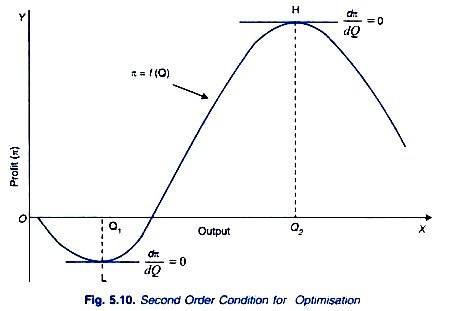
Consider again the case of profit maximisation explained above. A profit function curve such as the one drawn in Figure 5.10 may have both minimum point and maximum points. It will be seen from Figure 5.10 that point L represents the minimum point and H represents the maximum point of the profit curve. Important thing to note is that at both minimum point L and maximum point H, first order condition, that is, first derivative dπ/dQ be zero is satisfied at both points, L and H, corresponding to OQ1 and OQ2 levels of output.
However, at point L profits are minimum and at point H profits are maximum. It is with the help of the second derivative of a function that we can distinguish between maximum and minimum along a function. Whereas the first derivative measures the slope of a function, the second derivative measures the slope of the first derivative. Thus, in case of profit function, whereas first derivative, dπ / dQ measures the slope of the profit function curve. That is, marginal profit, its second derivative, d2π / dQ2 measures slope of the marginal profit function curve.
ADVERTISEMENTS:
Since the second derivative of a function when measured at the maximisation level is always negative and when measured at the minimisation level is always positive, it can be used to distinguish between points of maximum and minimum. For example, if the second derivative in our profit function curve is negative, it implies that profits are maximum at the level where first derivative is equal to zero.
On the other hand, if the second derivative at a point on a profit function where first derivative is zero is positive, it shows profits are in fact minimum rather than maximum. It can be easily known from having a look at Figure 5.10. It will be seen from this figure that up to point L, marginal profit (dπ / dQ) that is, slope of the total profit curve, is negative and has been causing the total profits to fall (in fact, up to L, due to negative marginal profits loses have been increasing. At point L, marginal profit I and thereafter it becomes positive and therefore it will causes the total profit to increase.
Hence, point L beyond which the second derivative (i.e. the slope of the first derivative) is positive, and since profits will be increasing beyond this point, it cannot be point of maximum profits.
ADVERTISEMENTS:
Now consider point H on the total profit corresponding to output level OQ2. At point H, first derivative (dπ / dQ) is again equal to zero but after that marginal profit dπ / dQ becomes negative as the slope of total profit curve is negative as output is expanded beyond Q2. This causes the total profits to fall. This shows that point H at which first derivative, dπ / dQ is zero and also beyond which second derivative (d2π / dQ2), that is, slope of the first derivative becomes negative is indeed the point of maximum profit.
To conclude, we get a following general test for maximum and minimum:
(1) If the second derivative d2y / dx2 of a function is negative (< 0) at the point where the first derivative (dy / dx) is zero, it will represent a point of maximum.
(2) If the second derivative (d2y / dx2) of a function is positive (> 0) at the point where first derivative is zero, it will represent a point of minimum.
ADVERTISEMENTS:
Coming back to our profit function (π = – 100 + 160 Q – 10 Q2) in which case the first derivative is zero at 8 units of output, we test for the sign of second derivative. Thus,
dπ / dQ = 160 – 20Q
d2π / d2Q = -20.
Thus, we find that at 8 units of output profits will in fact be maximum.
3. Minimisation Problem:
In some decision making problems the objective of a manager is to minimise the objective function. For example, efficiency in the use of resources requires that a firm should produce at the minimum possible cost per unit of output.
For example, the following average cost function of a firm is given:
ADVERTISEMENTS:
AC = 25,000 – 180Q + 0.50Q2
A manager is interested to find what level of output the firm will minimise its average cost. This can be obtained by differentiating the AC function with respect to output (Q) and setting it equal to zero, Thus
d(AC)/ dQ = – 180 + 1.0Q
Setting it equal to zero and solving for Q we have:
-180 +1.0 Q = 0
Q = 180
ADVERTISEMENTS:
Applying the second order condition to ensure whether it is really minimum we take the second derivative of AC function
d2(AC)/ dQ2 = + 1.0
Since second derivative of AC function is positive, d2 (AC)/ dQ2 > 0, output of 180 units of output is one that minimises average cost of production.
4. Multivariate Optimisation:
When a dependent variable is a function of many independent variables we use the concept of a partial derivative. Partial derivatives are therefore used to find optimal solution to maximisation or minimisation problem in case of two or more independent variables. Rules for finding maximisation and minimisation problems are the same as described above in case of one independent variable. To maximise or minimise a multivariate function we set partial derivative with respect to each independent variable equal to zero and solve the resulting set of simultaneous equations.
Consider that a firm is producing two products X and Y. Its profit function may be written as
π = f (X, Y).
ADVERTISEMENTS:
Consider a firm producing the two products whose function is given below
π = 50X -2X2 –XY-4Y2 +75Y
Where X and Y are two independent variables representing levels of outputs of two products. It is to decide what levels of output of the two products will maximise profits.
Differentiating the profit function with respect to X while holding Y constant we have
dπ/ dX = 50 – 4X – Y
Differentiating the profit function with respect to y while holding X constant we have
ADVERTISEMENTS:
dπ/ dY = – X – 8Y+ 75
For maximisation of profits we must set each partial derivative equal to zero and then solve the resulting set of simultaneous equations for optimal values of independent variables x and Y. Thus,
∂π/ dX = 50 – 4X- y= 0 ….(i)
∂π/ dy =75 – X – 8y = 0 ….(ii)
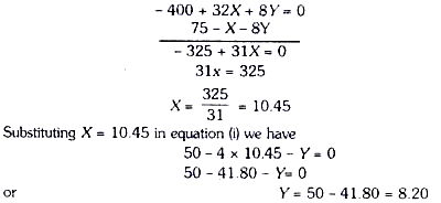
To solve the above two equations simultaneously we multiply equation (i) by – 8 and adding (i) and (ii) we have
Thus the firm will maximise profits of it produces and sells 10.45 units of product X and 8.2 units of product Y1.


