
Here is a compilation of essays on ‘Consumer Behaviour’ for class 9, 10, 11 and 12. Find paragraphs, long and short essays on ‘Consumer Behaviour’ especially written for school and college students.
Essay on Consumer Behaviour
Essay Contents:
- Essay on the Introduction to Consumer Behaviour
- Essay on the Assumptions of Consumer Behaviour under Cardinal Theory
- Essay on the Mathematical Derivation of Consumer Behaviour
- Essay on the Economic Interpretation of FOC
- Essay on the Price Effect as a Sum-Total of Substitution Effect and Income Effect
- Essay on the Hicksian Interpretation of Consumer Behaviour
- Essay on Choice Under Uncertainty
- Essay on the Modern Approach of Consumer Behaviour
Essay # 1. Introduction to Consumer Behaviour:
ADVERTISEMENTS:
Microeconomic theory tends to assume that individuals are the economic agents exercising the act of consumption, the decision to purchase goods and services. The consumer is assumed to choose among the available alternatives in such a manner that the satisfaction derived from consuming commodities (in the broadest sense) is as large as possible.
This implies that he is aware of the alternatives facing him and is capable of evaluating them. All the information pertaining to the satisfaction that the consumer derives from various quantities of commodities is contained in his ‘utility function’.
We assume that each consumer or family unit has complete information on all matters pertaining to its consumption decision. A consumer knows precisely what his money income will be during the planning period. ‘Utility’ refers to subjective satisfaction derived from consumption of commodities.
The 19th century economists, namely W. Stanley Jevons, Leon Walras and Alfred Marshall came up with the cardinal theory of consumer behaviour. They considered utility is measurable just as the weight of objects. The consumer is assumed to possess a cardinal measure of utility when he is able to assign every commodity, a number representing the amount or degree of utility associated with it.
ADVERTISEMENTS:
Under this theory, it is possible to measure marginal utility (MU) of a commodity, whereby by MU we mean a change in utility due to a change in per unit of consumption of a commodity. Another property is the existence of Law of Diminishing Marginal Utility (LDMU).
This means as a consumer keeps on consuming successive units of the same commodity, consumption of other commodities held fixed, marginal utility diminishes. Total utility increases at a decreasing rate for successive units of consumption of a particular commodity.
Essay # 2. Assumptions of Consumer Behaviour under Cardinal Theory:
(i) Utility is numerically measurable.
ADVERTISEMENTS:
(ii) Marginal utility is the unit of measurement of utility.
(iii) Marginal utility of money (or total budget) is constant.
(iv) The Law of DMU holds,
(v) Independence axiom holds.
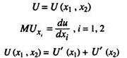
Total utility can be expressed as sum of utilities pertaining to each commodity separately. For example, let utility be a function of two goods x1 and x2, i.e.,
Cardinal theory of consumer behaviour also is helpful to explain the law of demand in the following ways:
Essay # 3. Mathematical Derivation of Consumer Behaviour:
Let U (x) be the utility from commodity X whose price is Px. Let N (x) be the net utility from x and λ be the marginal utility of money (assumed constant).
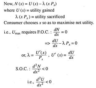
i.e., U”(x) < 0 which is true by the assumption of LDMU. Hence, utility can be maximised by finding optimal (indicating consumption bundles).
Essay # 4. Economic Interpretation of FOC:
Suppose that an individual purchases 1 unit of x. This leads to increase in utility by MUx On the other hand, utility loss is λPX. At the optimum these two must be equal, i.e., MUX – λPX.
Alternatively, we may give another type of economic interpretation of such an optimality condition. Suppose that an individual spends one additional unit of money on x. This leads to increase in utility by MUx/Px .
ADVERTISEMENTS:
On the other hand, utility loss is MUM = λ.
At the optimum, utility gained = utility sacrificed.
This implies that U'(x)/Px = λ or, U’(x) = λPx
Now, if, MUX > λ Px (additional 1 unit of x),
ADVERTISEMENTS:
then, MUx/Px > MUM (additional 1 unit of money spent).
Ultimately, the consumer incurs sacrifice of utility. Given the law of DMU, consumption of x rises and, therefore, MUX falls until equality between MUx and λPx holds. Hence once optimality has been reached, it is always possible for the consumer to find the optimal demand function.
For many economists in the last century, the assumptions on which the theory of cardinal utility was built were very restrictive. They reformulated the theory of consumer behaviour and named it ‘The Ordinal Theory of Utility’.
According to the ordinal theory, utility is no longer a measurable concept. What is required is the existence of a preference base such that an individual can rank the consumption bundles according to his preference ordering. Let us define two binary evaluations ‘preference to’ (symbolically P) and ‘preference between’ (symbolically I).
This preference ordering is among/ between ‘consumption bundles’, which refers to certain amount of different commodities. For example: X = {x1, x2,…, xn} is a consumption bundle consisting of, n commodities x1, x2, ……, xn.
The ordinal theory of utility is based on the following axioms of preference ordering:
ADVERTISEMENTS:
1. Completeness:
Let there be two consumption bundles X’ and X”. An individual can rank these bundles in the following mutually exclusive ways:
(a) X’ P X”, i.e., X’ is preferred to X”
(b) X” P X’, i.e., X” is preferred to X’
(c) X’ I X”, i.e., X’ is indifferent to X”
2. Transitivity:
ADVERTISEMENTS:
For three commodity bundles, the axiom of transitivity states that if X’P X” and X” PX'”, then automatically, X’ PX'”.
3. Non-Satiation:
If consumption bundle X’ contains more of at least one commodity and no less of other commodity compared to X” and X'”, it means more is better than less.
4. Strict Convexity of Preference Ordering:
Let X’ I X”. Let us suppose X'” a consumption bundle which is a weighted average of X’ and X”. In this case, X'” can be expressed as a convex combination of X’ and X”, i.e., X'” = αX’ + (1 – α) X” where 0 < α < 1.
Now, according to this axiom,
ADVERTISEMENTS:
X'” is preferred to both X’ and X”.
5. Continuity of Preference:
There exist a set of points in the consumption space which divides it into less preferred and more preferred areas such that these points are indifferent to one another. Once these assumptions or axioms are valid, it is easier to show consumer preferences in a commodity space as in Fig. 1 (in a two-dimensional or two-commodity framework).

In Fig. 1 we divided consumption space into four zones — I, II, III, IV. Due to the axiom of non-satiation it is observed that consumption bundle, XPY (X has more of x2 than Y for the same x1). Similarly, ZPY Hence all the points in zone I are superior to Y and all the points in zone III are inferior to Y.
The remaining two zones, viz., II and IV are important to draw indifference map as follows:
ADVERTISEMENTS:
A ray through origin, OH, passes through Zone II. All Space points on OP are inferior to Y but XPO i.e., somewhere between P and X where there is switch of preferences say point M. Successive drawings of such a ray through origin can make us safely assert that there is a point say M which is indifferent to X. Similar exercise can be carried out with Zone IV and joining these points like W, M, Y, T, we get a curve called Indifference Curve.
An indifference curve is a locus of points in a commodity space—or commodity bundles—among which the consumer is indifferent. Each point on an indifference curve yields the same utility as any other point on that indifference curve. The IC approach has been applied in areas of international trade and public finance, community (social) indifference curves (ICs and SICs) are used to show gains from trade.
Similarly, ICs are used to compare to the welfare effects of a lumpsum tax and a price distorting tax. IC approach including the Slutsky theorem is also used to show the effect of income tax on a worker’s labour-leisure choice. At times SICs are used to compare cost of living indices and then show the effects of price inflation.
We may now summarise the basic properties of indifference curves as follows:
1. IC is Downward Sloping:
In Fig. 2, along the IC, utility is constant. Therefore, when consumption of one commodity increases, given the level of other commodity, utility increases. But since total utility is constant, additional utility has to be sacrificed by reducing the consumption of other commodity. Hence IC is downward sloping.

2. ICs are Non-Intersecting:
In Fig. 3, CPB (since C has more of x1 than B for same x2). But CIA as both C and A lie in same IC, IC0. Again, BIA, as both B and A lie on same IC1.
... Therefore, by the axiom of transitivity, CIB (or BIC) which is not possible or gives contradictory results. Therefore ICs cannot intersect.

3. Higher ICs give Higher Utility:
It can be seen that BPA, as more of x2 is consumed in B than A for the same amount of x1. Hence all the points on IC1 are preferred to all the points on IC0, as it gives higher utility. Again, CPB as for same x2, more of x1 is consumed. Therefore, all points on IC2 are preferred to all points on IC0 and IC1 as it gives more utility. Higher IC gives higher utility (Fig. 4).

4. ICs are Convex to the Origin:
Axiom 4 leads to convexity of IC which implies diminishing MRS where by MRS we mean absolute necessary reduction in consumption of x1 due to additional consumption of x2 by one unit such that total utility is fixed (assuming two commodities x1 and x2 only)
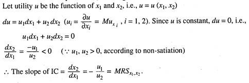
5. The Law of DMRS Holds:
This implies that due to the convexity of IC, as consumption of x1 increases successively by equal unit, fall of x2 declines, i.e., for constant utility x2 falls at a diminishing rate. Thus, MRS falls along an IC in Fig. 5.

Now we shall discuss about budget constraint and budget lines. The budget line is set off more commodity bundles than can be purchased, if the entire money income is spent.
Hence, budget constraint is given by following equation:
![]()
where m = total money income (assumed constant).
Pi = price of ith commodity
Xi = ith commodity, i = 1, 2,…, n
In a two-commodity framework, therefore, the budget constraint will be
m=p1x1 + p2x2
or, x2 = (m/p2 – p1/p2) x1 [This is indeed the equation of a downward sloping straight line.]
The solution of problem of maximisation of utility subject to the budget constraint is the main motive behind the theory of consumer behaviour.
Properties of Demand Functions:
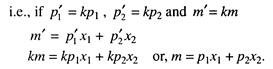
Demand functions are homogeneous of degree zero in prices and income which means that equi-proportional and unidirectional changes in prices and money income do not alter optimality condition. This homogeneity postulate suggests that the consumer is free from money illusion.
The Consumer’s Reaction to Income and Price Changes:
So long we assumed that the consumer maximizes his welfare subject to two constraints:
(i) A fixed level of money income and
(ii) A fixed set of commodity prices.
Now we may relax the assumptions one by one and do some comparative statics exercise. Changes in m, with P1/P2 held constant. We first consider the consumers’ reaction to a change in his money income holding the prices of the two purchasable goods constant. A change in the consumer’s money income causes a parallel shift of the budget line with no change in slope as shown in Fig. 6.

Consumers’ initial equilibrium is point E. Every time his income increases the budget line shifts F and G are the corresponding equilibrium points. The locus of all the equilibrium points is called income consumption curve. In the Fig. 6 both x1 and x2 are normal goods.
If x1 is inferior the ICC will be backward bending and if x2 is inferior it will be forward falling. See (Fig 7). If consumption of a good falls as income rises, then such a commodity is called inferior goods. So one important prediction is that if the consumer spends all his income on two goods, both cannot be inferior at the same time.

The relation between money income and quantity consumed is explained by a function is known as the Engel’s curve. Now we allow the price of one of the two goods to fall. Suppose that of x1 falls. In this case the budget line becomes flatter and the consumer is able to reach higher indifference curves and enjoy more utility or satisfaction, thus improving his level of welfare.
So every time P1 falls, the consumer moves to higher IC and reaches a new equilibrium point. The locus of successive equilibrium points is the price consumption curve (PCC) which shows the consumer’s reaction to a single price change which changes the price ratio, i.e., p1/p2.

There are two uses of PCC. First, we can derive the consumer’s demand curve for a commodity from the PCC. According to the ordinal approach, the demand curve for a normal good is downward sloping due to price effect which has been decomposed by Hicks and Slutsky into two parts, namely, substitution effect and income effect. The slope of the demand curve depends on the relative strength of the two effects which, in turn, depends on the nature of the commodity under consideration.
From the PCC we can predict price elasticity of demand (e) by using the total outlay method.
Three points will be noted in the context:
(i) If PCC is downward sloping, demand for x1 is price elastic.
(ii) If PCC is horizontal, demand for x1 is unitary price elastic.
(iii) If PCC is upward sloping, demand for x1 is price inelastic.

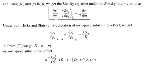
Essay # 5. Price Effect as a Sum-Total of Substitution Effect and Income Effect:
From the Marshallian demand curve (constant money income demand curve) it is not possible to explain the price effect because Marshallian approach is based on LDMU, i.e., cardinal theory. It was John Hicks and E. Slutsky who decomposed the price effect into two parts. Thus, two new concepts of demand curve have emerged, namely,
(i) Real income constant demand curve (the Slutsky demand curve)
(ii) Total utility constant demand curve (the Hicks demand curve)
We shall now construct Marshallian demand curve and compensated demand curve for a normal good in a two-commodity framework.
From the price effect such derivation of the demand curve for x1 is as follows:
Let initial budget line be AS in Fig. 10(a) for price p1, corresponding equilibrium x1 at E0 is x1. Hence for price p1, x1 is plotted in Fig. 10(b). If p1 falls slope of budget line falls and hence AB becomes flatter. The budget line becomes AB’. The consumer reaches higher utility level on IC2 and new equilibrium x1 is x1M. Plotting this in Fig. 10(b) and joining E0 and EM in Fig. 10(b), we get the negatively sloped demand curve for x1 which is the Marshallian demand curve, DM.

We will construct DH and DS for same initial conditions as the one we considered while drawing the Marshallian demand curve. Let price of x1, p1 fall from p1o to p1’. For Hicksian demand curve we consider budget line, CD tangent to initial IC0 implying constant utility level even as new price ratio P’1/P2 and hence parallel to AB’. Because of movement from E0 to EH, x1 rises from x1 to x1H. This is purely substitution effect, and joining E0 and EM we get Hicksian demand curve DH.
If we follow the Slutsky approach, we can make the following two Predictions:
(i) Perfect Substitutes:
If two commodities are perfect substitutes like blue and black ink for a colour blind person the IC will be a straight line with PE = SE and IE = 0.
(ii) Perfect Compliments:
If two commodities are perfect complements like left and right shoe SE = 0 Thus, PE = IE. For Slutsky demand curve we consider budget line C’ D’ , which passes through initial equilibrium point E0 implying that consumer is just enough to purchase initial equilibrium commodities even at new price ratio P’1/P2, hence parallel to AB.
This hypothetical budget line is thus to the right of CD and hence consumer reaches higher IC, IC1. Consumption of x1 rises, hence when plotted in 10(b), we see that DS is flatter than DM. The movement from ES to EM is the income effect.
The substitution effect is always negative because the entire IC approach is based on the of substitution which suggests that the consumption of one commodity is always at the expense of the other but IE is negative in case of normal good, if we consider change in real income. Thus in case of a normal good the negative income effect reinforces the negative, SE so as to make the price effect very strong in this case and the demand curve is relatively flat.
In case of an inferior good, IE is positive but less-strong than the substitution effect. So the price effect is still negative but less strong than that in the case of a normal good. In case of a Giffen good, which is essentially a price phenomenon, the positive income effect is stronger than the negative substitution effect so as to cause price effect to be positive. This is one of the exceptions to the empirical law of demand. These points are summarized in Table 1.

An important aspect of ordinal theory is the derivation of Slutsky Equation. This is done in the mathematical appendix.
Essay # 6. The Hicksian Interpretation of Consumer Behaviour:
Hicks define own-price substitution effect in terms of constant utility.
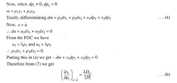
This is own-price substitution effect according to Hicks. Under Slutsky interpretation, money income is so adjusted that individual can purchase initial consumption bundle even at new prices.
Hence dm = x1dp1 + x2dp2 -dm + x1dp1 + x2dp2 = 0

This is own-price substitution effect, according to Slutsky. Now let us derive the income effect.
From (7) we get

The Homogeneity Property of the Demand Function own-price substitution effect is always negative. Modem economists like K. Lancaster and L.R. Klein have generalized the homogeneity property and have emerged with the conclusion that the result holds even in situations when only representative consumer purchases different goods instead of two. In fact, due to interrelationships of demand the quantity demanded of each commodity is a function of ‘n’ absolute prices and the money income of the buyer. So the constrained optimisation problem here is
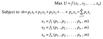
Now to derive the homogeneity property of the demand functions we have to express the quantity demanded of each commodity as a function of relative prices and real income. If there are ‘n’ absolute prices, there will be (n – 1) relative prices. So we can rewrite the demand functions as
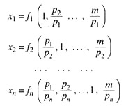
In this case, if all absolute prices and the money income get doubled at the same time, the relative prices and real income will remain constant and there is no reason why the consumer’s purchase plan will be altered. It is a tribute to the Nobel laureate economist Paul A. Samuelson who developed the revealed preference approach to show that if we eliminate the income effect of a decrease in p, it is still possible to derive the downward sloping demand curve for x1 from the actual choice of consumer in the market place.
Revealed preference is a relation that holds between the bundle that is actually demanded at some budget and bundles that could have been demanded at that budget. For example, when we say X = X (x1 , x2) is revealed preferred to Y = Y (y1 , y2), we are claiming that X is chosen when Y could have been chosen, i.e., p1x1 + p2x2 ≥ P1Y1 + P2Y2.
Samuelson retains the two main assumptions of the IC approach, namely, rationality and consistency and has provided a scientific basis of the theory of the consumer demand in terms of two axioms of revealed preference, namely, weak axiom of revealed preference weak axiom of revealed preference (WARP) and strong axiom of revealed preference (SARP). WARP implies that, if (x1, x2) is directly preferred to (y1, y2) and the two bundles are not same, then it cannot happen that (y1 y2) is directly revealed preferred to ( x1, x2).
This implies that if (x1, x2) is purchased at price (p1, p2) and (y1, y2) is purchased at (q1, q2), then if initially, P1x1 + p2x2 ≥ p1y1 + p2y2 then must be the case that q1y1 + q2y2 ≥ q1x1 + q2x2, i.e., X is purchased when Y was affordable and when y was purchased, x must not be affordable. Fig. 11 satisfies the WARP.

According to SARP, if (x1, x2) is revealed preferred to (y1, y2) (either directly or indirectly) and (y1, y2) is different from (x1, x2) then (y1, y2) cannot be directly or indirectly revealed preferred to (x1 x2). Likewise, in the ordinal theory under revealed preference approach it can be proved that substitution effect is always negative. Let prices be given by P° when a consumer purchases a commodity bundle X° when X’ was affordable. This means X° is purchased at P° when X’ was affordable. This is possible only when,
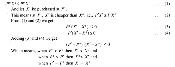
Obviously, for such inequality to hold, we have assumed that P’ ≠ P°. Hence there must be strict inequality i.e. (P’ – P°) (X’ – X°) < 0 which implies and proves that the substitution effect is always negative. It may however, be noted that two approaches, namely, the indifference curve and revealed preference approach are not mutually exclusive. Economists like W.J. Baumol and Hal Varian have shown that it is possible to derive the consumers’ indifference map by using the revealed preference approach.
Essay # 7. Choice under Uncertainty:
So far we have a certain environment; now let us consider choice under uncertainty.
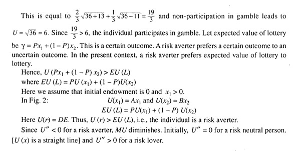
Let L = (x1 , x2 , p) denote a lottery, i.e., a consumer receives price x1 with probability p and x2 with probability (1 -p). Let M0 denote initial endowment. According to the expected utility theorem, we have EU (L) =pU (M0 + x1) + (1 -p) U (x2 + M0) where U is a function of money value and is cardinal. The utility is additive separable in x1 and x2 and is linear in p and (1 -p).
Let the utility function be U = √M and initial endowment be M0 = 36. Let us consider a gambler, in which individuals coins 13 with probability 2/3 and loses 11 with probability 1/3. We needed to examine whether the individual participates in gambler or not. For this we must calculate expected utility from the gambler.

Essay # 8. Modern Approach to Consumer Behaviour:
An alternative approach to the theory of consumer demand was pioneered by K. Lancaster. He argued that goods are demanded as their characteristics. It is these characteristics that yield utility. Thus, we may consider three different goods say sugar, honey and saccharixe. But they may have only two characteristic, viz., sweetness and calories. If a new sweetener is produced we analyse it not as a new good but as one better that has the same characteristics.
Thus, compared with traditional analysis, the new approach has two advantages:
(i) We can study the introduction of new goods,
(ii) We can study the effects of changes in quality.
Comparison with traditional approach:
In the traditional theory, the consumer’s indifference curves are given in terms of the original set of goods. Now if a new good is introduced in the market we have to introduce a whole new set of indifference curves or surfaces. All the information in the preference about old set of goods is discarded.
In terms of the new approach we can make an insightful analysis of consumer choice. In the real commercial world many of the so-called new goods are actually the same as the old goods with the characterisation of different proportions.
Thus, if we consider the preferences in terms of characterisation we can analyse introduction of new goods very easily. We do not have to discard any old set of preferences as worse. If new goods appear in the market with new characteristics, we have to introduce a new set of preferences.
A major advantage of the characteristic approach is that it permits the analysis of many goods. At times the number of goods is considerably higher than the number of characteristics. Furthermore, once we think in terms of characteristics we have to consider substitution effect which is different from the substitution effect of the traditional theory.