Propensity to Consume or Consumption Function

Propensity to Consume or Consumption Function:

To construct macroeconomic models as developed by Keynes, it is necessary to have a clear understanding of the consumption function. In fact, the concept of the consumption function is the ‘heart’ of the Keynesian analysis.

The concept of propensity to consume (i.e., willingness to consume) or the so-called consumption function is based on a ‘funda­mental psychological law’ which states that “men are disposed, as a rule, and on an average, to increase consumption as their income increases but not by as much as the increase in their income.”

Although many factors influence aggregate consumption, aggregate disposable income or national income is, by far, the most important one in the Keynesian theory. So, here we will concentrate on the relationship between planned consumption and income—the consumption function.

Keynes’ consumption function has the following attributes:

i. Consumption is a stable function of disposable income, i.e., C = f(Y).

ii. Consumption is assumed to vary directly with disposable income. As disposable income rises, consumption rises.

iii. The rate of increase in consumption is less than the rate of increase in income. In Keynes’ terminology, the value of the marginal propensity to consume (MPC) is less than one (i.e., MPC < 1).

iv. MPC is less than the average propensity to consume (APC) in the short run (MPC < APC).

Here consumption expenditure is a planned one, but not the actual one. Thus, in a consumption function, a relationship between disposable national income (that is, income after tax payments) and planned consumption expenditure is established.

Before elaborating on Keynes’ consumption function, let us explain the terminologies of APC and MPC.

(a) APC and MPC:

APC is the ratio of consumption to income. It is the proportion of income that is consumed. It is worked out by dividing total consumption expenditure (C) by total income (Y).

Symbolically,

APC = C/Y

MPC measures the response of con­sumption spending to a change in income. It is the ratio of change in consumption to a change in income. It is worked out by dividing the change in consumption by the change in income.

Symbolically,

MPC = ∆C/∆Y

Suppose, disposable national income rises from Rs. 100 crore to Rs. 200 crore. As a result, consumption spending rises from Rs. 125 crore to Rs. 200 crore.

Thus,

MPC = 200-125/200-100

= 75/100 = 0.75 = 3/4

In this example, MPC = 3/4. The economic meaning is that if national income rises by four rupees, consumption spending would increase by three rupees and the remainder one rupee would be saved. Note that, in this example, the value of MPC is positive but less than one (0 > MPC < 1).

Since at zero level of income, consumption is positive, so MPC must always be positive. Further, since increase in consumption is less than that of increase in income, the value of MPC must be less than one.

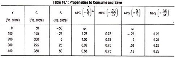
The relationship between planned consumption expenditure and disposable income is presented in Table 10.1 in terms of a hypothetical data.

Table 10.1 tells us that when income is zero, consumption is positive (Rs. 50 crore). But as income increases, consumption rises. Further, as the rise in consumption is less than the rise in income, APC declines.

However, since the rate of increase in consumption is less than the rate of increase in income, the value of MPC is always less than one (here 0.75). At the same time, MPC is always positive because consumption is positive even if income is zero. Finally, the table suggests that MPC < APC.

Consumption function equation:

The relationship between consumption spending and income is usually explained in an equation form:

C = a + bY (a > 0; 0 < b < 1)

Here C and Y represent consumption and national income, respectively. This equation indicates that consumption is a linear function of income since it is the equation of a straight line. In the equation, ‘a’ stands for autonomous consumption—consumption that does not vary with the changes in national income. This part of consumption spending is independent of the level of income.

Its value is positive in the sense that consumption is always positive, even if income is zero, ‘b’ is the behavioural coefficient or the MPC. This part of consumption is called ‘induced’ consumption. According to Keynes, MPC is always positive but less than one. Here ‘b’ is the slope of the consumption function. Thus, MPC is the slope of the consumption line.

(b) Consumption Function in a Graphi­cal Form:

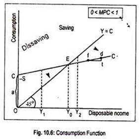
The consumption function equation can be represented in terms of Fig. 10.6 where we measure income on the horizontal axis and planned consumption expenditure on the vertical axis. All points on the 45° line show that the values measured on the two axes are equal (i.e., Y = C).

The line CC’ is the consumption line which cuts the vertical axis at some positive point. Positive vertical intercept (a > 0) of the consumption function implies that planned consumption expenditure exceeds income at very low levels of income. The line CC’ is upward rising.

This means that, as income rises, consumption rises. Such consumption is called induced consumption. At an income level of OY₀, CC’ line coincides with the 45° line. That is to say, at point E, income equals consumption. Such equality of income and consumption is called breakeven point.

To the left of point E, say at OY₁ income level, as consumption exceeds income there occurs negative saving or dissaving. This means that people consume more than their income, i.e. they spend their past savings. Actually, to the left of point E, CC’ line lies above the 45° line and to determine dissaving we have used -S sign in Fig. 10.6.

On the other hand, to the right of E, i.e., at an income level of OY₂, income exceeds consumption (and, hence, CC’ line lies below the 45° line) and positive saving occurs. As people do not spend their entire income on consumption, the rest is saved.

One can determine APC and MPC from the position or the location of CC’ line and slope of the CC’ line, respectively. At zero income, APC = ∞. As income rises, APC declines but it never becomes zero. To determine the value of MPC, we have chosen two points f and d on the line CC’. As we move from f to d, income rises (A Y) by ft and consumption rises (∆C) by dt.

Thus, MPC = ∆C/∆Y = dt/ft = slope of the line CC’. Its value is less than unity since the rate of increase in consumption (dt) is less than the rate of increase in income (ft). As CC’ is a straight line, MPC remains constant at all levels of income.

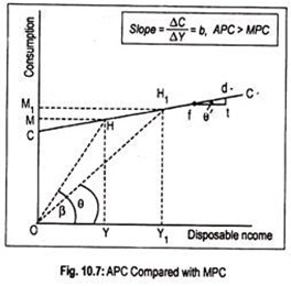
Though MPC remains constant as income rises, APC continuously declines on a straight line consumption function. This may be explained by examining Fig. 10.7. Let us consider point H on the line CC’. Correspon­ding to this point, income is OY and consumption is OM.

Thus, APC at point H is:

APC= OM/OY

Now consider the dashed lines β and θ drawn from the origin. Lines such as these are called rays. The slope of the ray β is equal to the tangent of the angle β and is, therefore, equal to OM/OY. Thus, the slope of the ray to point H is the APC at point H.

Similarly, the slope of the ray to point H₁ is the APC. In other words, the slope of the dashed lines OH and OH₁ represent APCs at points H and H₁, respectively. Since the slope of the ray OH₁ is less steep than that of the slope of the ray OH, APC declines as income rises.

To calculate MPC, one must take into account the slope of the consumption line CC’ between points, such as f and d, in Fig. 10.7. By inspection, we can see that tan β or tan θ is greater than tan θ’. This suggests that APC > MPC. So we can conclude that the coordinates at any point on a consumption line give us the value of APC and the slope between any two points gives us the value of MPC.

Consider Fig. 10.6 again. At zero income APC = ∞; to the left of point E, APC > 1; at point E, APC = 1; and to the right of point E, APC < 1.

On the other hand, 0 < MPC < 1 (i.e., double inequality). On a straight line consumption function, MPC remains constant at all levels of income. Thus, the Keynesian consumption function of the short run variety shows that APC > MPC. We can prove this in the following way. The equation of the linear consumption line is C = a + bY.

From this equation, one obtains:

APC = C/Y = a/Y + b,

and MPC = b.

Thus, APC > MPC by the amount a/Y. Or MPC < APC implies b < a/Y + b which implies 0 < a/Y

We have already said that Keynes’ consumption function is a short run one and the relationship between consumption and income is a non-proportional one in the sense that MPC < APC.

However, a long run consumption function shows a proportional relationship between income and consumption. Because of this proportional relationship, MPC = APC. The long run consumption function starts from the origin. Its functional form is thus C = bY.

Saving Function or Saving Propensity:

As propensity to consume refers to willingness to consume so does propensity to save refers to willingness to save. Saving is the difference between income and planned consumption, i.e.,

S = Y – C

Saving function is derived from the consumption function. Planned saving is a function of aggregate disposable income, i.e.,

S = f (Y)

Keynes’ saving function has the following characteristics:

i. Saving is a stable function of disposable income.

ii. Saving varies directly with disposable income.

iii. The rate of increase in saving is less than the rate of increase in income. At very low levels of income as well as at zero income, since consumption is positive, saving must be negative. As income increases, dissaving vanishes and saving becomes positive. In Keynes’ terminology, this feature suggests that the value of the marginal propensity to save (MPS) is positive but less than one.

(a) APS and MPS:

Before describing the Keynesian saving function, it is better to equip ourselves with the concepts of average propensity to save (APS) and MPS.

The complementary concepts of APC and MPC are APS and MPS, respectively. APS is the proportion of income devoted to savings. It is obtained by dividing total saving by total income, i.e.,

APS = S/Y

Or, APS = Y – C/Y (S = Y – C)

Table 10.1 suggests that when consump­tion exceeds income there occurs negative saving, so is the value of APS. When income and consumption are equal, APS becomes zero. Now, if income increases, APS would tend to rise.

MPS is the change in saving consequent upon a change in income. It is the proportion of any addition to income that is used for saving. Symbolically,

MPS = ∆S/∆Y

The value of MPS is always less than one. In Table 10.1, MPS has been assumed to be 0.25, i.e., 1/4. This means that an increase in disposable national income of Rs. 4 will lead to an increase in saving by one rupee. Here MPS is constant at all levels of income.

Saving Function Equation:

As consumption function equation is a linear one, so saving function must be a linear one:

S = Y – C = Y-(a + bY) [^..^. C = a + bY]

Or, S = – a + (1 – b)Y [0 < (1- b) < 1]

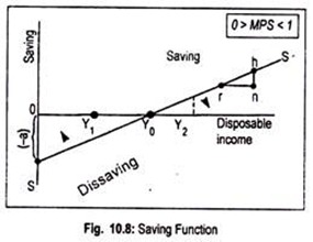
This is the saving equation in a linear form, ‘-a’ indicates negative saving represented by the vertical (negative) intercept as shown in Fig. 10.8. In terms of this figure, we find that saving function SS’ starts from the negative quadrant. Here (1 – b) is the MPS. If we know MPC (i.e., b) we can obtain MPS (i.e., 1 – b).

Saving Function in a Graphic Form:

Fig. 10.8 depicts a linear saving function SS’. This function is a rising saving function. To indicate negative saving at zero level of income (i.e., negative saving represented by [-a]), saving function starts to rise from the vertical axis below the origin. Now, as income rises, saving rises and, therefore, dissaving declines.

At OY₀ level of income, (since income equals consumption) saving is zero. That is why saving line at that level of income cuts the horizontal axis. To the left of OY₀ level of income, as saving is negative, SS’ line lies below the horizontal line. To the right of OY₀ level of income, as saving is positive, SS’ line lies above the horizontal line.

The slope of the saving function is given by the MPS. To calculate MPS, we have chosen two points r and h on the line SS’. As we move from r to h, national income (∆Y) rises by rn amount and saving (∆S) rises by nh amount.

Thus,

MPS = ∆S/∆Y = nh/rn = slope of the SS’ line.

The value of MPS is always positive but less than one.

(a) Relationship between APC and APS and MPC and MPS:

A part of income is consumed while another portion of it is saved by people. So, if we know the value of APC or MPC, we can easily find out the value of APS or MPS.

How APS is calculated from APC as:

APC = C/Y

APS = S/Y = Y – C/Y = 1 – C/Y

(^..^. S = Y – C)

Or, APS = 1 – APC

As APC and APS are complementary terms their sum must be equal to one.

We know that

Y = C + S

Now, dividing both sides of this equation by Y, we obtain

Y/Y = C/Y + S/Y

1 = APC + APS

Or, APS = 1 – APC

When APC rises (or falls) APS falls (or rises). When APC = 1, APS must be equal to zero, and when APC = 0, APS = 1. But since APC can never be zero, so APS can never be equal to one. It must be less than one.

We calculate MPS from MPC. To do so, first we show that the sum of MPC and MPS is equal to one and MPS must be (1 – MPC). This is because income is always equal to consumption plus saving. Or

Y = C + S

Now, suppose, income changes to ∆ Y. As a result, both consumption and saving change to ∆C and ∆S, respectively, i.e.,

∆Y = ∆C + ∆S

Dividing both sides of this equation by ∆ Y we get

∆Y/∆Y = ∆C/∆Y + ∆S/∆Y

Or, 1 = MPC + MPS

or, MPS = 1 – MPC

When MPC rises (falls) MPS must fall (rise) in such a manner that their sum becomes equal to one.