Measuring Price Elasticity of Demand: 4 Methods

The following points highlight the top four methods used for measuring elasticity of demand. The methods are:- 1. The Percentage Method 2. The Point Method 3. The Arc Method 4. Total Outlay Method.

1. The Percentage Method:

The price elasticity of demand is measured by its coefficient (E_p). This coefficient (E_p) measures the percentage change in the quantity of a commodity demanded resulting from a given percentage change in its price.

Thus

Where q refers to quantity demanded, p to price and Δ to change. If E_P>1, demand is elastic. If E_P< 1, demand is inelastic, and E_p= 1, demand is unitary elastic.

With this formula, we can compute price elasticities of demand on the basis of a demand schedule.

 

Let us first take combinations B and D.

(i) Suppose the price of commodity X falls from Rs. 5 per kg. to Rs. 3 per kg. and its quantity demanded increases from 10 kgs.to 30 kgs.

Then

This shows elastic demand or elasticity of demand greater than unitary.

Note:

The formula can be understood like this:

Δq = q₂-q₂ where q₂ is the new quantity (30 kgs.) and q_i the original quantity (10 kgs.).

ΔP = p₂-p₁ where p₂ is the new price (Rs.3) and p_l the original price (Rs. 5).

In the formula, p refers to the original price (p₁) and q to original quantity (q₁). The opposite is the case in example (i) below, where Rs. 3 becomes the original price and 30 kgs. as the original quantity.

(ii) Let us measure elasticity by moving in the reverse direction. Suppose the price of Arises from Rs. 3 per kg. to Rs. 5 per kg. and the quantity demanded decreases from 30 kgs. to 10 kgs.

Then

This shows unitary elasticity of demand.

Notice that the value of Ep in example (ii) differs from that in example (i) depending on the direction in which we move. This difference in the elasticities is due to the use of a different base in computing percentage changes in each case.

Now consider combinations D and F.

(iii) Suppose the price of commodity X falls from Rs. 3 per kg to Re.lper kg. and its quantity demanded increases from 30 kgs. to 50 kgs.

Then

This is again unitary elasticity.

(iv) Take the reverse order when the price rises from Re. 1 per kg. to Rs. 3 per kg. and the quantity demanded decreases from 50 kgs. to 30 kgs.

Then

This shows inelastic demand or less than unitary.

The value of E_p again differs in this example than that given in example (iii) for the reason stated above.

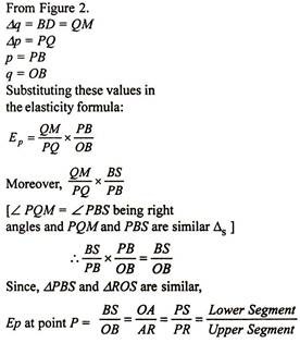
2. The Point Method:

Prof. Marshall devised a geometrical method for measuring elasticity at a point on the demand curve. Let RS be a straight line demand curve in Figure. 2. If the price falls from PB ( = OA) to MD ( = OC), the quantity demanded increases from OB to OD.

Elasticity at point P on the RS demand curve according to the formula is:

EP = Δq/Δp x p/q

Where Δq represents change in quantity demanded, Δp changes in price level while p and q are initial price and quantity levels.

With the help of the point method, it is easy to point out elasticity at any point along a demand curve. Suppose that the straight line demand curve DC in Figure. 3 is 6 centimeters. Five points L, M, N, P and Q are taken on this demand curve. The elasticity of demand at each point can be known with the help of the above method. Let point N be in the middle of the demand curve. So elasticity of demand at point.

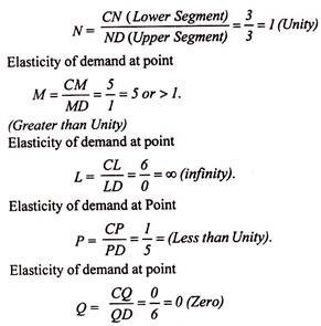
We arrive at the conclusion that at the mid-point on the demand curve, the elasticity of demand is unity. Mov­ing up the demand curve from the mid-point, elasticity be­comes greater. When the demand curve touches the Y- axis, elasticity is infinity. Ipso facto, any point below the mid-point towards the A’-axis will show elastic demand. Elasticity becomes zero when the demand curve touches the X -axis.

3. The Arc Method:

We have studied the measure­ment of elasticity at a point on a demand curve. But when elasticity is measured between two points on the same de­mand curve, it is known as arc elasticity. In the words of Prof. Baumol, “Arc elasticity is a measure of the average responsiveness to price change exhibited by a demand curve over some finite stretch of the curve.”

Any two points on a demand curve make an arc. The area between P and M on the DD curve in Figure. 4 is an arc which measures elasticity over a certain range of price and quantities. On any two points of a demand curve, the elasticity coefficients are likely to be different depending upon the method of computation. Consider the price-quantity combinations P and Mas given in Table. 2.

If we move in the reverse direction from M to P, then

Thus the point method of measuring elasticity at two points on a demand curve gives different elasticity coefficients because we used a different base in computing the percentage change in each case.

To avoid this discrepancy, elasticity for the arc (PM in Figure 4) is calculated by taking the average of the two prices [(p₁ + p₂ )^½] and the average of the two quantities [(q, +q₂ )^½]. The formula for price elasticity of demand at the mid-point (C in Figure 4) of the arc on the demand curve is

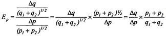
On the basis of this formula, we can measure arc elasticity of demand when there is a movement either from point P to M or from M to P.

From P to M at point P, p₁ =8, q₁ = 10, and at point M, p₂ = 6, q₂ = 12.

Applying these values, we get

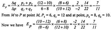
Thus whether we move from M to P or P to M on the arc PM of the DD curve, the formula for arc elasticity of demand gives the same numerical value. The closer the two points P and M are, the more accurate is the measure of elasticity on the basis of this formula.

If the two points which form the arc on the demand curve are so close that they almost merge into each other, the numerical value of arc elasticity equals the numerical value of point elasticity.

4. The Total Outlay Method:

Marshall evolved the total outlay, or total revenue or total ex­penditure method as a measure of elasticity. By comparing the total expenditure of a purchaser both before and after the change in price, it can be known whether his demand for a good is elastic, unity or less elastic.

Total outlay is price multiplied by the quantity of a good purchased: Total Outlay = Price x Quantity Demanded. This is explained with the help of the demand schedule in Table.3.

(i) Elastic Demand:

Demand is elastic, when with the fall in price the total expenditure increases and with the rise in price the total expenditure decreases. Table.3 shows that when the price falls from Rs. 9 to Rs. 8, the total expenditure increases from Rs. 18 to Rs. 24 and when price rises from Rs. 7 to Rs. 8, the total expenditure falls from Rs. 28 to Rs. 24. Demand is elastic(Ep > 1) in this case.

(ii) Unitary Elastic Demand:

When with the fall or rise in price, the total expenditure remains unchanged, the elasticity of demand is unity. This is shown in the table when with the fall in price from Rs. 6 to Rs. 5 or with the rise in price from Rs. 4 to Rs. 5, the total expenditure remains unchanged at Rs. 30, i.e., Ep = 1.

(iii) Less Elastic Demand:

Demand is less elastic if with the fall in price, the total expenditure falls and with the rise in price the total expenditure rises. In Table 3 when the price falls from Rs. 3 to Rs. 2, total expenditure falls from Rs. 24 to Rs 18, and when the price rises from Re. 1 to Rs. 2. the total expenditure also rises from Rs. 10 to Rs. 18. This is the case of inelastic or less elastic demand, Ep < 1.

Table 4 summarises these relationships:

The measurement of elasticity of demand in terms of the total outlay method is explained in Fig. 5 where we divide the relationship between price elasticity of demand and total expendi­ture into three stages.

In the first stage, when the price falls from OP₄ to OP₃ and to OP₂ respectively, the total expenditure rises from P₄ E to P₃ D and P₂ C respectively. On the other hand, when the price in­creases from OP₂ to OP₃ and OP₄, the total expenditure decreases from P₂ C to P₃ D and P₄ E respectively.

Thus EC segment of total expenditure curve shows elastic demand (Ep > 1).

In the second stage, when the price falls from OP₂ to OP₁ or rises from OP₁ to OP₂, the total expenditure equals, P₂C = P₁B, and the elasticity of demand is equal to the unity (Ep = 1).

In the third stage, when the price falls from Op₁ to Op, the total expenditure also falls from P₁ B to PA. Thus with the rise in price from OP to Op₁, the total expenditure also increases from PA to P ₁B and the elasticity of demand is less than unity (Ep < 1).