
The below mentioned article provides a study note on the cost function.
Economies and Diseconomies of Scale:
The behavior of long run average total cost to the changes in scale [by increasing all inputs to raise the level of output of the firm] can be studied by estimating the economies and dis-economies of scale. The economies of scale in total cost can be estimated by fitting the total cost function to the data on total cost and output of the firm.
The term ‘Economies of Scale’ refers to the situation where the proportionate change in the total cost of the production will be relatively smaller than the proportionate change in total output, all else equal. In other words, it is a situation where long run average total cost declines with the increase in output of the firm.
ADVERTISEMENTS:
The total cost function will be hypothesized as follows, all else equal:
C = f (Q)
Where
C = Total cost
ADVERTISEMENTS:
Q = Output
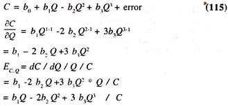
The rate of change in total cost per a unit change in output is marginal cost and the ratio of total cost of the production to the output is an average cost. The ratio of marginal cost to average cost is, technically, known as the elasticity of total cost of the production to the changes in output [EC.Q]
E C.Q= ΔC/ΔQ * Q/C
If E C.Q is less than unity, then there will be economies of scale [Increasing returns to scale] It is a situation where long run average total cost declines with the increase in output of the firm
ADVERTISEMENTS:
If E C.Q is more than unity, then there will be diseconomies of scale [Decreasing returns to scale] It is a situation where long run average total cost increases with the increase in output of the firm
If E C.Q is unity, then there will be neither economies of scale nor dis economies of scale [Constant returns to scale] It is a situation where long run average total cost will be constant with the increase in output of the firm.
Polynomial Cost Function:
In empirical research the following form of third degree polynomial total cost function will be estimated by ordinary least squares method.
ADVERTISEMENTS:
If EC.Q< 1, then there will be economies of scale in the cost of production
If EC.Q > 1, then there will be diseconomies of scale in the cost of production
ADVERTISEMENTS:
If EC.Q = 1, then there will be neither economies of scale nor diseconomies of scale in the cost of production
Polynomial Cost Function-Estimates of Economic Relationships:
The following data [Table 14.1] on cost of the production and output are considered to estimate the polynomial cost function [Cubic Cost Function].

ADVERTISEMENTS:
Visual Plot:
The pair values of total cost and output are plotted [Figure 14(A)]. The shape of the cost curve is found to be in compliance with the theory.

The regression results of the polynomial cost function are presented in table 14.2.


ADVERTISEMENTS:
The estimates of coefficients of the above function are in conformity with the theoretical expectations.
B0 > 0
B1 > 0
b2 < 0
b3 > 0
Therefore the marginal cost curve [MC = 51.13095 – (1.584524*2*Q + (0.0I6667*3*Q2) ] has a typical U shape and average cost [AC = (1920.000/Q) +51.13095 – (1.584524* Q) + (0.016667* Q2) ] curve has an L shape or an inverse J shape . It should be noted that the U shaped cost curves of the theory may not represent reality.
ADVERTISEMENTS:
Therefore various forms of cost functions such as linear. Quadratic [Second degree], polynomial [third degree] etc., will be fitted to the data in cost studies [See appendix] The values/values/shapes of marginal and average cost curves based on the third degree polynomial regression model [Equation (115)] are given in table 14.3 and figure 14(B) and figure 14(C)


The elasticity of total cost of production with respect to production is less than unity [0.44507675] showing the presence of economies of scale. The numerical value of elasticity of total cost of production with respect to production illustrates that a one percent increase in total production leads to increase the total cost of production by 0.44507675 percent only. In other words the long run average total cost of the production declines [LRATC CURVE] with the increase in the scale of production.
The actual values, fitted values and residuals are given in table 14.4. The visual plot of the same is also furnished in figure 14(D). The numerical value of the durbin watson is a matter of concern though the actual and fitted curves move together closely [Table 14.4 and figure 14(D)] with low drift.


The mean and other summary statistics pertaining to total cost and output are given in table 14.5.

Appendix:
Linear Cost Function:
The data given in table 14.6 are considered to fit the linear cost function and quadratic cost function by OLSM.
ADVERTISEMENTS:
The specification of a Linear Cost Function will be as follows:
C = b0 + b1Q + error………. (116)


The regression results [Table 14.7]show that the regression coefficient of output [Q] is a marginal cost and constant at all levels of output [though the scale of output increases].
The actual and fitted cost curves based on the linear cost function are shown below:

Quadratic Cost Function:
The quadratic cost function is also fitted to the same data [Table 14.6].
The specification of a quadrate cost function will be as follows:
C = b0 + b1Q + b2Q2 + error………………. (117)
The regression results of the quadratic cost function are given in table 14.8

The Regression results of the quadratic cost function [Table 14.8] show that [though the coefficients are not significant] the marginal cost goes on increasing with the increase in the scale of output. The actual and fitted cost curves based on he regression results of the quadratic function are shown in figure 14(F).
