Consumption Function: Economics Notes on Consumption Function | Econometrics

The below mentioned article provides notes on consumption function.

The functional relationship between the aggregate consumption expenditure and aggregate disposable income is known as the aggregate consumption function, all else equal.

This can be shown as follows:

Y₁ = f [X]

Where

Y₁ = Aggregate consumption expenditure,

X = Aggregate disposable income

The rate of change in consumption expenditure per a unit change in disposable income is termed as an mpc [marginal propensity to consume] That is ΔY_t/ΔX_t = Y_t – Y_t-1,/Y_t – X_t-1

Where

X_t = Income in current [t] year

X_t-1 = Income in previous [t-1] year

Y_t = Consumption expenditure in current year

Y_t-1 = Consumption expenditure in Previous year

The numerical value of mpc can be calculated between two points of time. But in the empirical studies the numerical value of mpc is being estimated over a period of time or across the units [Households] at a point of time by applying the regression method.

Linear Aggregate Consumption Function:

If the relationship between Consumption expenditure and disposable income is linear, then the specification will be as follows:

Y₁ = b₀ + b₁X + error……………. (20)

The numerical values of b₀ and b₁ in the equation will be estimated by OLS method under the main assumption that there is one-way causation between income and consumption expenditure, i.e., If Y depends on X or X influences Y, then X will be an exogenous variable.

If such relationship exists then the consumption expenditure will always be influenced by the disposable income, all else equal, evincing the fact that disposable income will be exogenous. The derivative of Y₁ with respect to X, dY₁/dX, b₁, is an mpc whose value will be less than unity as the increase in the consumption expenditure will be smaller than the increase in disposable income leaving some margin for savings.

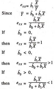
The responsiveness of consumption expenditure to the changes in disposable income (elasticity of y₁ with respect to X or ratio of marginal propensity to consume [mpc] to Average propensity to consume [apc]) will be estimated as follows:

e_y.x = dY₁ / dX.X / Y₁

In the linear [consumption function] regression model, the numerical value of the elasticity will be estimated as follows: dY₁/dX .X/Y₁ = b₁ X / Y₁ which can be b₁* X_i/Y_1i or b₁ * mean value of X/mean value of Y₁ or b₁ * ∑ X/∑Y₁.

The value of elasticity of consumption expenditure, if estimated at different values of Y₁ and X, varies from point to point change in X and Y₁. An increase in X inflates the value of elasticity of consumption expenditure with respect to disposable income and a decline in X deflates the value of elasticity of consumption expenditure with respect to disposable income, all else equal.

In the empirical studies the value of elasticity would be evaluated at the mean value of Y₁ and X. Hence it is known as average elasticity. If the numerical value of elasticity of consumption expenditure with respect to disposable income is more than unity, then [1] MPC will be higher than APC [2] The proportion of consumption expenditure in disposable income [APC] increases with an increase in disposable income [3] The proportionate change in consumption expenditure will be higher than the proportionate change in disposable income and [4] The growth rate in consumption expenditure will be higher than the growth rate in disposable income.

If it is less than unity, then [1] MPC will be lower than APC [2] The proportion of consumption expenditure in disposable income [APC] declines with an increase in disposable income. [3] The proportionate change in consumption expenditure will be lower than the proportionate change in disposable income and [4] The growth rate in consumption expenditure will be lower than the growth rate in disposable income.

If it is unity, then [1] an MPC will be equal to APC [2] The proportion of consumption expenditure in disposable income [APC] will be constant with an increase in disposable income. [3] The proportionate change in consumption expenditure will be equal to the proportionate change in disposable income and [4] The growth rate in consumption expenditure will be equal to the growth rate in disposable income.

The probable value of the elasticity of aggregate consumption expenditure with respect to disposable income can be inferred on the basis of the sign of the intercept of the simple linear consumption function.

Y = b₀ + b₁X + error

If b₀ is less than zero [negative], then the size of the elasticity will be more than unity. If b₀ is more than zero [positive], then the size of the elasticity will be less than unity. If it is zero, then the size of the elasticity will be unity.

 

 

 

 

 

 

 

 

 

 

 

 

The linear consumption function, Y = b₀ + b₁X + error, will be estimated with the underlying assumption that there is one-way causation between Y and X.

It should be noted that this assumption will not be satisfied because of two way causation between Y and X [Y depends on X and X depends on Y] as shown below:

It is well known fact that income is sum of consumption expenditure and Investment.

X = Y₁ + Y₂; Income = [Consumption expenditure] + [Investment]

Where

Y₁ = Aggregate consumption expenditure

Y₂ = Non-Consumption Expenditure [Investment]

X = Disposable income which is total of Y₁ and Y₂

This will be specified as follows:

X = c₀+ c₁Y₁+ c₂Y₂ + U

In the above equation if Y₁ = b₀ + b₁X + U is substituted, then we get the following:

X = c₀+ c₁ [b₀+ b₁X] + c₂Y₂+ U

X = c₀+ c₁b₀+ c₁b₁X + c₂ Y₂+ U …………………….. (21)

Thus, the covariance between X and error term [U] will not be zero, i.e., X is dependent variable on random variable [U] i.e., consumption expenditure depends on income and income depends on consumption expenditure. Thus, there will be two- way causation between X and Y₁.

Therefore, the numerical value of mpc will be biased [upward biased]. In order to reduce the bias in mpc, both two-stage least squares method [TSLSM] and indirect least squares method [ILSM] would be used in the empirical studies.

Estimation of an MPC by Two-Stage Least Squares Method:

At the first stage the income [X] will be regressed on non- consumption expenditure [Y₂] as shown below:

X = b₀+ b₁ Y₂ + error………………. (22)

The trend values of X [estimated values: X_c] will be estimated with the help of the values of b₀ and b₁ estimated by OLS method.

At the second stage, the trend values of income [X_e] will be considered as the independent variable to regress Y₁ on X_e as follows:

Y₁ = d₀ + d₁X_c + error………………. (23)

The co-variance [correlation] between X_e and U[estimated values of X and random variable] will be close to zero. Thus in two stage least squares method the assumption of zero co-variance between X_e and U [random variable] will to some extent be satisfied to reduce an upward bias in MPC.

Estimation of an MPC by Indirect Least Squares Method:

In the Indirect Least Squares method, the consumption expenditure [Y₁] will be regressed on non-consumption expenditure [instrumental variable] as shown below:

Y₁ = b₀ + b₁Y₂ + error………………….. (24)

Then the income [X] will be regressed on non- consumption expenditure [Y₂] as shown below:

X = c₀+ c₁Y₂+ error……………………….. (25)

Intercept in the consumption function = c₀/c₁

Slope [mpc]in the consumption function = b₁ /c₁

Thus, b₁/c₁ will be unbiased mpc in the consumption function

Power Consumption Function or Log Linear Consumption Function:

In empirical studies, the Power function is also widely considered to estimate an MPC.

The specification of a power model will be as follows:

y = b₀ X₁^b1 …………….(26)

Where

b₁ is constant elasticity of aggregate consumption expenditure with respect to income as shown below:

dY/dX₁ = b_1.b₀X₁^b1-1

= b_1.b₀X₁^b1.X₁^-1

= b₁Y / X₁ which will be an mpc and varies with the change in Y and X.

The elasticity of consumption expenditure with respect to disposable income will be estimated as follows:

e_y.x = dY/dX.X/Y

In the above model [power function] by substituting dY/dX = b₁Y/X in the elasticity equation [e_y.x= dY/dX.X/Y] we get the following:

e_YX = b₁Y/X. X/Y = b₁ which is known as constant elasticity of aggregate consumption expenditure with respect to disposable income.

Distributed Lag Consumption Function:

In empirical studies on Consumption Function the Distributed lag-models [Dynamic Models] are used to estimate both the short-run and long-run consumption functions through the partial adjustment mechanism.

The long-run/desired level/equilibrium level consumption function will be specified as follows:

Y_t*= b₀+ b₁X_t+ U_t ……………………(27)

Where

Y_t* is desired or fully adjusted level [long run or optimal level] of aggregate consumption expenditure which is not observable.

Therefore, the above equation will be estimated through the partial adjustment mechanism [Nerlovian Model or Partial adjustment model] as shown below:

Y_t – Y_t-1 = δ[Y_t^* – Y_t-1]…………..(28)

Where

Y_t – Y_t-1 = actual change in consumption expenditure

Y_t^* – Y_t-1 = desired change in consumption expenditure

δ is the coefficient of adjustment whose values will be in between zero and one. If it is 1, then the actual change in consumption expenditure will be equal to desired change in consumption expenditure i.e., actual consumption expenditure adjusts to the desired level of consumption expenditure in the same period [instantaneously].

If it is zero, then there will be no change in actual consumption expenditure since the actual consumption expenditure in time will be equal to consumption expenditure observed in the previous period [t – 1] i.e., Y_t = Y_t-1. If it is less than 1, then the adjustment to the desired level of consumption expenditure is likely to be incompleted because of friction, rigidities etc..

In order to estimate, the above equation will be simplified as shown below:

Y_t = δ [Y_t^* – Y_t-1] + Y_t-1

Substituting the partial adjustment model in the above equation, we get the following:

 

 

 

 

 

 

 

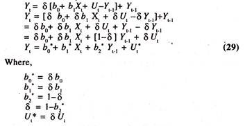
The above equation is referred to as the short-run consumption function.

Where

δ Y_t/δ X_t= b₁ is the short-run MPC. The short run [Time is not long enough for consumers to adjust completely to the changes in income] average elasticity of consumption expenditure with respect to disposable income will be estimated as follows

SRE = δ Y_t/δ X_t * X_t/Y₁ = b₁* mean of X_t/mean of Y_t

The long run [Time is enough for consumers to adjust completely to the changes in income] consumption function will be obtained by deflating the short run consumption function by δ [coefficient of adjustment] and deleting X_t-1 as shown below:

 

 

Where

b₁^*/δ is long run MPC.

The long run elasticity [LRE] will be obtained by dividing the short run elasticity [SRE] by δ, coefficient of adjustment as shown below:

LRE = b₁*X_t/Y_t/δ

= b₁* X_t/Y_t.1/ δ

It should always be noted that the numerical values of the long run MPC and long run elasticity of aggregate consumption expenditure with respect to income will be relatively higher than the corresponding short run MPC and short run elasticity. Further, it should be noted that the value δ = 1 –b₂* depicts the extent of discrepancy between actual change and desired change in consumption expenditure that can be deleted in that period.

Similarly, in log linear [power] function, both the long- run and short-run MPC and elasticity will be estimated by using Nerlovian’s Partial Adjustment Mechanism [Model] as shown below:

 

 

 

 

 

 

 

 

 

 

 

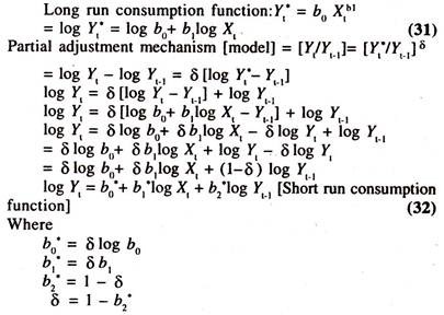
The derivative of log Y_t with respect to log X_t ∂ log Y_t/∂ log X_t,is b₁, known as the short run constant elasticity of consumption expenditure with respect to disposable income.

The short run mpc, (SRMPC), ∂Y_t/∂X_t = b₁^* Y_t/X_t

The long run MPC will be estimated as follows

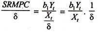
The long run average elasticity [e_yt.yt] will be estimated as follows:

SR e_yt.xt/δ = b₁/δ

Differential Marginal Propensity to Consume:

The constant marginal propensity to consume for two different time periods [i.e., the pre and post economic reform periods or two different regions/categories/groups] can be worked out using the following model.

Y = b₀ + b₁D + b₂X + b₃ (D. X)

Where,

Y = Aggregate consumption expenditure

X = Aggregate Disposable income

D = Dummy variable, which takes 0 (zero) for pre- economic reform period and 1 (one) for Post-economic reform period.

(D X) = An interaction variable to capture the interaction effect of changes in aggregate disposable income and presence of attribute [D = 1]

The constant mpc for pre economic period [D – 0] can be worked out as follows:

dY/dX = b₂

b₂ is an MPC for the pre-economic reform period. The sign will be positive and size will be less than unity.

The MPC for post-economic reform period can be worked out as follows:

d Y/dX = b₂+ b₃

Where, b₃ is the differential MPC during post-economic reform period.

If the sign of b₃ is significantly positive then there will be an upward shift in the magnitude of MPC during post- economic reform period.

If the sign of b₃ is significantly negative then there will be a downward shift in the magnitude of MPC during post- economic reform period.

If the sign of b₃ is statistically insignificant, then there will be no shift/change in the magnitude of MPC during post- economic reform period. This shows that the MPC will be same both in pre and post-economic reform periods.

Consumption Function—Estimates of Economic Relationships:

The following data [Table 3.1] on private final consumption expenditure [Rs.crore] at constant prices [Y] and gross domestic product [income] at market prices [X] are considered for estimating consumption function.

Visual Plot:

The consumption expenditure and income series move together in the same direction [Figure-3(A)]

The regression results of the linear consumption function [Table 3.2] show that the regression coefficient of income, which is known as constant mpc, is significantly positive and less than unity. According to this value one can infer that if income increases by one unit/one crore, then consumption expenditure would increase by 0.606 units/crore.

The sign of the intercept is positive showing the presence of positive consumption expenditure [trend value] in the absence of income. Further it can be inferred that the probable value of elasticity of consumption expenditure would be less than unity as the sign of the intercept in the linear consumption function is positive.

The value of elasticity of consumption expenditure estimated at the mean values of Y and X: 0.60630*[438842.1/322195.0] is 0.8258 showing that a one percent increase in income leads to increase the consumption expenditure by 0.8258 percent per annum, all else equal.

The presence of two-way relationship between consumption expenditure and income creates a bias in mpc. In order to reduce the extent of bias the two stage least squares method [TSLSM] with an instrumental variable [S = X-Y] is adopted to estimate the aggregate consumption function. The results are furnished in Table 3.4.

Xe = Estimated (Trend) Values of X = 0.146544.0 + 2. 505832 (S)

S = Instrumental Variable

Where

S = X -Y

X = Observed Income

Y = Observed Consumption Expenditure

The results of the consumption function based on the two stage least squares method show that the value of mpc, 0.6009, is marginally smaller than the mpc estimated by OLS method. In estimating an mpc by TSLSM, first, the trend values of income have been estimated by regressing the income on savings [Non-consumption expenditure], [X = 146544.0 + 2.505832S] which is an exogenous variable.

Then the consumption expenditure is regressed on estimated values [trend values] of income[y = b₀ + b1 X_e]. The regression results based on indirect least squares method are furnished in Table 3.5 and Table 3.6 respectively.

The values of intercept and mpc by ILSM are 58481.151 [intercept/slope in the regression of X on S: (1465544/2.505833) Table 3.6] and 0.60093 [slope in the regression of Y on S [Table 3.5]/slope in the regression of X on S [Table 3.6] (1.5058833/2.505833)] respectively, i.e. Y = 58481.15 + 0.60093 X

The results of the log linear consumption function [Table 3.8] based on the data given in table 3.7, show that the regression coefficient of log income is significantly positive and its value is 0.837.

This is constant elasticity of consumption expenditure with respect to income and explains that a one percent increase in income leads to increase the consumption expenditure by 0.8366 percent, which is less than unity. The value of mpc is 0.65 [estimated at geometric mean values of Y and X :0.84*(287098.32/372190.09)] explaining that a one unit increase in income leads to increase the consumption expenditure by 0.65 units.

The regression results of the distributed lag linear consumption function [Table 3.10] based on the data given in table 3.9 show that the regression coefficient of income is significantly positive but its value is low and less than unity. This could be due to the serious problem of multicollinearity between the independent variables. This can be assessed from correlation matrix.

The figures furnished in 3.11 table show that the variables X_t and Y_t-1 are strongly correlated. The value of the coefficient of partial adjustment [1 – 0.712] is 0.288 showing that every year the discrepancy between actual change in consumption expenditure and desired change in consumption expenditure can be reduced to the extent of 0.28 units.

If the distributed lag linear consumption model is not found to be suitable to the data points, then the other form of the distributed lag model such as log linear distributed consumption lag model will be considered. The data points [generated] given in table 3.12 are considered for fitting this model. Regression results of log linear distributed lag consumption function are given in table 3.13.

The regression results of log linear distributed lag consumption function show that the regression coefficient of log income is 0.50 showing that a one per cent increase in income leads to increase the consumption expenditure by 0.50 percent per annum, all else equal.

The coefficient of consumption expenditure lagged by one year is statistically significant showing the presence of significant lag in the adjustment of consumption expenditure to its desired level.

The value of the coefficient of partial adjustment or speed of adjustment [1-0.40] is 0.60 implying that about 60 percent of the discrepancy [disequilibrium] between actual change and desired change in consumption expenditure can be eliminated in a year, all else equal.

The degree of correlation between X_t and Y_t-1 can be assessed from correlation matrix furnished in table 3.14. It should be noted that Durbin ‘h’ statistic is appropriate to detect the presence of serial correlation between independent variables in distributed lag models.