Theory of Economic Growth – An Overview

Theory of Economic Growth – An Overview !

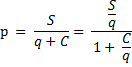
Introduction:

The Classical Theory of Growth can be explained in a simple way — given a certain amount of labour (assuming labour theory of value), at a certain level of production, wages will be paid to each worker according to the level of subsistence and any surplus (TP – TC = Total Surplus) accumulated by the capitalist Such accumulation will increase the demand tor labour and, with a given population, wages will tend to rise.

As the wage exceeds temporarily the level of subsistence, the population will increase according to the Malthusian Theory of Population. With a growth of population, the supply of labour will increase and wages will again fall back to the subsistence level.

The dynamics of growth ends as the law of diminishing returns sets in and wages eat up the whole production — leaving no surplus for accumulation, expansion and growth of population. The ‘magnificent dynamics’ ends not with a bang but a whimper as Fig. 18.1 shows.

The vertical axis measures TP and the horizontal axis measures L = Labour and OW line is a subsistence wage line. With ON₁ population, production is OP, wage per unit is N₁W₁ and surplus or profit is N₁E₁, when TP = Wages + Profits.

The emergence of a surplus engenders accumulation which leads to an increase in the demand for labour. Wages rise to E₁N₁ since the demand for L rises with accumulation but population, and, thus L supply remains constant at ON₁. But once the wages are above the level of subsistence, i.e. N₁E₁ > N₁W₁, growth of population is stimulated to ON₂.

Once the population is ON₂, a surplus emerges again, i.e. W₂E₂, as wages are driven back to the level of subsistence and the whole process is repeated until the economy reaches a point E where the stationary state is reached. As W = TP, there is no surplus and the day of doom is reached. If technical progress is introduced (a shift of TP to TP’), then the day of doom is postponed, but not eliminated.

Limitations of the Model:

(1) The role of technical progress has been underestimated in the model. The experience has shown that the role of DR, as the pointer to the day of doom, has certainly diminished.

(2) The iron law of wages, which suggests that wages cannot be above the subsistence level because the Malthusian Law of Population has been discredited as the sole-explanation of wage determi­nation. The iron law of wages is based only on supply, whereas wages are determined both by demand and supply. It does not take into account the role of trade union on wage determination.

(3) The Malthusian Theory of Population Growth has been found to be misleading in the light of the experience of economic-development of the economically advanced European countries. The Malthusian argument that, whenever wages are above the subsistence level, people like to have more babies rather than other things seems to be unacceptable, both logically and empirically.

(4) The classical model seems to be too simplistic to account for the complex factors which influence growth.

Keynesian Theory and the Classical Theory:

It is significant to observe that, in classical theory, money is a ‘veil’ and has nothing to do with the determination of real factors like output and employment; money plays no role in the equilibrium analysis of value and distribution in the classical system, whereas in the Keynesian model money tends to influence the equilibrium values of output and employment. Later, Patinkin tried to integrate value and monetary theory by introducing the real balance effect.

One of the main sources of conflict between the Keynesian and classical theories lie in the way the difference between demand for and supply of money should be corrected. In the classical theory, an increase in money supply will raise unwanted cash holding and, since a rational individual does not hold money for its own sake, excess money would be spent on goods and services, pushing the price upwards, with a given level of output.

The mechanism is explained with the help of the quantity theory: MV = PT, where M = quantity of money, V = Velocity, P = Price Level and T = total transaction. It is assumed that V and T are unlikely to change substantially in the short-run. In such a situation, an expansion of M will have a direct and positive impact on prices. The critics, however, have argued that, if either V or T or both change with the change in M, then the direct relationship between M and P is unlikely to hold.

To this ‘new monetarists’ point out that, as long as the demand for money remains stable, an expansion of M will always lead to a rise in prices, though the effect may not be seen instantaneously. At a higher price the expansion of money supply would be consistent with ordinary transaction demand (k) which is assumed to be fixed proportion of income (Y), or M = kY.

In the Keynesian theory, an expansion of money supply will raise bond prices and reduce interest rate, increase the level of investment, output and employment and perhaps lead to a secondary effect on prices. Should there be excess capacity, the effect on prices of a rise in money supply will be even less. If we are concerned with an underemployment situation, prices should not be affected so long as the supply of output with respect to money supply is elastic. Thus, the effect could well be on income, output and employment.

Marxist Theory of Economic Growth:

Marx rejected some principal features of the Classical theory of economic growth and offered his own theory within a socio-historical framework in which economic forces play a major role. In Marxist theory, the law of diminishing returns has been discarded because Marx believed that the Classical theory of Stationary State was actually a creation of human actions rather than the end product of a natural, immutable law. For a similar reason, Marx also castigated the Malthusian theory of Population.

Marx looked at economic development from a social and historical stand­point. Each stage of economic growth was regarded as the product of Hegelian dialectics of a game of contradictions where a thesis created its anti-thesis and the conflict between the two produced a synthesis. Marx emphasised that, with capitalism, social relations of production are much more important than an exchange relations between goods.

The social character of labour has been stressed in particular. Marx argued that labour productivity ‘is a gift, not of nature, but of history embracing thousands of centuries’. However, the Marxist concept of relations of production is rather vague. It has been interpreted as an ‘organic whole’ characterized by labour organisation and skill, the standing of labour in society, technological and scientific knowledge and its use in a certain environment.

In the Marxist analysis, these ‘relations of production’ determine the socio-cultural set-up of a society. Marx believed that capitalism would not end up in a quiet classical ‘stationary’ state; rather, it would break up with a ‘bang’ ‘when the expropriators are expropriated’. Here we shall only analyse the economic views in the Marxist theory.

The Marxist model of economic growth depends on some major dynamic ‘laws’:

(1) The law of capital accumulation, which says that the prime desire of the capitalists is to accumulate more and more capital.

(2) The law of falling tendency of the rate of profit which plays a crucial role in the breakdown of the capitalist system.

(3) The law of increasing centralisation and concentration of capital, which tells us that, with the growth of capitalism, cut-throat competition among capitalists will lead to the annihilation of the smaller firms by bigger ones, which will lead to the growth of monopoly and concentration of economic power.

(4) The law of increasing ‘pauperization’ which implies the growth of the misery of the working class with the advancement of capitalism, reflected in wages being tied to the subsistence level coupled with a rise in the proportion of unemployed people — or, what Marx called the ‘industrial reserved army of labour’— made possible by the substitution of capital for labour in the process of technical change.

The simultaneous working of these laws would generate contradictory forces, which would eventually sharpen the class conflict between capitalists and workers or between ‘haves’ and ‘have-not’s’. Capitalism would face a violent death in the final confrontation, when the expropriators would be expropriated. Hence, Marx gave the clarion call: ‘workers of the world unite’, as they have nothing to lose except their ‘chain’ and ‘the whole world to conquer’.

The Marxist notion of the falling tendency of the rate of profit plays a crucial role in the whole process of change and can now be illustrated. According to Marx, the value of a commodity (W) is given by the sum of ‘constant capital’ (c) + the ‘variable capital’ (q) + the ‘surplus value’ (s).

If the working day consists of 8 hours and only 4 hours are required to produce a commodity for subsistence then for the remaining 4 hours, the worker is producing a surplus value, which is expropriated by the capitalists. More formally, W = c + q + s and X = s/q where x is the rate of surplus value or the rate of ‘exploitation’. Thus, in the above example,

4 hrs/4 hrs = 100% = X

The rate of profit (P) in the Marxian analysis is given by

Let S/q = X, i.e. the rate of exploitation, and c/q = J or the ‘organic composition of capital’. Then we have p = X/1 + J .Now, it is clear that, if X remained constant, P and J would be inversely correlated. A rise in J would take place as capitalism developed with continuous accumulation. Also, capitalists would substitute capital for labour whenever wages tended to rise above the subsistence level to maintain their rate of profit.

The process would lead to higher unemployment among the working class and sharpen the polarization of forces. On the other hand, the crisis of capitalism would be reflected in the periodic fluctuations of growth and a falling tendency of the rate of profit, which would lead to cut-throat competition among the capitalists which, in turn, would lead to monopoly. Eventually, the conflict between the ‘immiserized proletarians’ and the capitalists would toll the death-knell of capitalism.

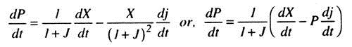
It is interesting to observe that the falling tendency of the rate of profit may not always be seen within an economic system. This can easily be demonstrated within the Marxist model. We have P = X/1 + J. Differentiating P with respect to time we get

Note that the profit rate will rise if the rate of exploitation rises more rapidly than the organic composition of capital. Even if the rise in the organic composition of capital is higher than that of the rate of exploitation, whether or not profit will fall depends on the difference between dx/dt and the product of profit rate and dj/dt.

For profit rate to fall, Pdj/dt (which is negative) must be greater than dx/dt. But a fixed rate of exploitation and an increase in capital intensity may not go together because a rise in organic composition of capital would raise labour productivity which would either raise the rate of exploitation or raise real wages. Inevitably, the internal consistency of the Marxist model has been questioned.

Further, a rise in the organic composition of capital could increase the rate of profit with an increase in productivity and a change in technology. Under such circumstances, the intensity of competition among capitalists declines. Technical progress may be neutral or even labour-using. Thus, the rise in the industrial reserve army of labour and a fall in the wage share in national income may not occur.

Other criticisms usually leveled against Marxist model may also be briefly mentioned. It is contended that Marx’s correlation between the growth of the average firm size and an increase in the degree of concentration need not always happen. However, the proportion of unemployment has increased in recent decades.

Empirically, wage share of national income in most developed economies remained fairly constant for a long lime and this phenomenon seems to have weakened the Marxist law of increasing pauperization. On the other hand, the Marxist prediction about the increasing concentration and centralisation of capital is not rejected. However, the rise in the output-capital ratios in developed economies probably reflects the growth of both accumulation and real wages, a phenomenon which Marx probably did not envisage within the strict framework of his analysis.

Rostow’s ‘Stage’ Theory of Development:

This theory states that the transition of an economy from being less developed to developed is possible through a series of steps. The most important of these is the so-called ‘take off stage when resistance to change in traditional values and, in the social, political and economic institutions of an underdeveloped economy is finally overcome and modern industries begin to expand. The theory may be criticised for viewing development as simply a matter of higher saving and investment ratios.

Saving and Investment:

Physical capital has always been at the centre of economic development. In order to invest, the country must save or, else, must have access to foreign saving through loans and aid. If domestic saving is the prerequisite for capital accumulation, then attention must focus on policies to promote saving.

Saving does depend on the availability of saving instruments — a banking system that offers convenient deposit services. There is evidence that extreme financial instability interferes with saving. When the return on saving becomes negative one of three things happens: households reduce their savings or they shift their saving abroad or they accumulate their saving in unproductive assets, such as gold. The financial environment for saving is thus an important factor in channeling saving from households to investing firms.

In addition to the private sector, the government affects national savings through its budgetary policies. It can also draw foreign savings to finance investment. A developing economy can tap foreign savings in three ways. One possibility is that, foreign firms invest directly in a country. The second way is that a country can tap foreign resources by borrowing in the world capital market or from institutions, such as the World Bank. Third possibility is that a country may receive foreign aid from industrialised countries.

The importance of these three sources of external saving has varied over time and between countries. But, there is no doubt that external saving can supplement domestic saving as it always has done. Of course, foreign saving is all the more important the lower the per capita income.

The amount of saving, whatever, may be its source, determines how much investment will take place in a country. But the productivity of investment may vary widely. The larger differences in productivity of investment across countries focuses attention on development policies and strategies that affect the efficiency of resource utilisation.

Harrod-Domar Growth Model:

This model assumes that:

(a) The economy is closed with no government. Thus, the condition for equilibrium is that, planned investment is equal to planned savings;

(b) There are only two factors of production, Labour(L) and Capital (K)and there is no technical progress;

(c) Labour is homogeneous, measured in its own units and grows at the constant natural rate of growth, n.;

(d) There are constant returns to scale. This means that, if both L and K are increased by a given proportion, output also increased by that proportion.

(e) Savings (S) are a fixed proportion of income (Y). That is, S = sY where s is both APS and MPS. Investment (I) is autonomous and there is no depreciation

(f) The potential national income (Y_P) is proportional to the quantity of K and L. Thus, we can write L = uY_P and K = vY_P, where u is a constant capital-output ratio and u is a constant labour-output ratio. This is a fixed proportional production function with L-shaped isoquant as in Fig. 18.2. Both K and L have to be employed in fixed proportions: as the Fig. 18.2 shows, increased capital and labour from OK₁ and OL₁ to OK₂ and OL₂ increased output from Q₁ to Q₂ (from A to B). Increasing only one of the factors would keep output unchanged (from A to C).

In Fig. 18.3, we start from equilibrium A and the initial investment I₁ which is equal to 5 at the income level OY₁ Over time, the investment adds to the capital stock and so increases the economy’s potential output, say to OY₂. The following analysis shows what the increase in potential output (∆Y_P) will be: K = vY_P, thus, ∆K = v∆Y_P. But ∆K + I₁, so we have ∆Y_P = I₁/ v……. (1)

The new level of income, OY₂, will be an equilibrium Y if AD increases. Assuming that the C and S functions are stable, thus, increase in demand must come from an increase in I. Investment must rise to l₂ as in Fig. 18.3, where l₂ intersects the savings line at Point B where OY₂ is an equilibrium income.

As the new K from this extra I comes into operation, potential output will rise yet again, say to OY₃. For this to be an equilibrium Y, investment must rise again — and so on as the growth-process continues.

This is Harrod’s warranted rate of growth (g_w) which can be derived as follows: ∆Y = I/v (from equation 1). In equilibrium, we have I = S = sY.

By substitution ∆Y = sY/v. Rearranging, ∆Y/Y = s/v = g_w. This is the rate of growth of output required to keep the economy in equilibrium at its potential output level. It is Harrod’s warranted rate of growth. For example, suppose v = 4 and that the savings proportion, s = 0.2. The warranted rate of growth (g_w) would be g_w = 0.2/4 = 5%.

This means that 5% growth would be necessary to keep the potential and equilibrium output levels equal. Thus, the warranted rate of growth can be increased by policies designed to increase the propensity to save or to reduce the capital-output ratio by measuring the productivity of K.

In this model output can only grow at the warranted rate, s/v, if sufficient labour is made available. It is assumed that the labour force is growing at the constant rate n; if n > s/v, the warranted rate can be achieved but will lead to an increasing rate of unemployment; if n < s/v, the actual rate of growth will fall short of warranted rate and unemployed capital will be created. Thus, for an equilibrium growth path which maintains full employment of both L and K, the following condition must be satisfied: n = s/v. That is, warranted rate of growth must be equal to the natural rate of growth.

Unfortunately, s, v and n are all constants in the Harrod-Domar model and unrelated to one another. It would be a complete ‘fluke’ if n = s/v. We can conclude that the equilibrium rate of growth in this model is highly unlikely to be achieved automatically. Furthermore, when s/v ≠ n, the economy will either experience increasing labour unemployment (when s/v < n) or increasing under-utilisation of K (when s/v > n). When such disequilibrium occurs, there are no forces generated to restore the equilibrium growth path. In other words, the equilibrium in the Harrod-Domar model is an unstable, or ‘knife- edge’, equilibrium.

Criticism:

(1) The model’s major drawback is its dependence on an inflexible production function, where no substitution is possible between L and K. It is more realistic to assume that there is some substitution between labour and capital. If there is some factor substitution; the isoquant map will have the more familiar shape as in Fig. 18.4. It is now possible to increase output from Q₁ to Q₂ by increasing the capital stock from OK₁ to OK₂, keeping the labour force unchanged, or by increasing the labour force from OL₁ to OL₂, keeping the capital stock unchanged.

With a production function of this kind, the capital-output ratio (v) can vary. Suppose that the warranted and natural rate of growth are not equal. As an example, let s/v > n; this means that the capital stock is growing faster than the labour force and also faster than output. Consequently, the capital-output ratio will rise and so s/v will fall. This tendency will continue until s/v = n again, which is the steady state growth; all economic variables grow at the constant proportional rate which is equal to the natural rate of growth.

Then the economy is on its long-run equilibrium growth path. This view, that any s/v ≠ n will be corrected by a change in u, is the basis of the so-called neo-classical growth model, which will be developed in the latter sections. In the meantime, we shall see some of the interesting uses of the model in the national planning.

Uses of Harrod-Domar Growth Model in National Planning:

The central point in the growth theories developed by Harrod-Domar is concerned with the existence of a unique equilibrium rate of growth which may or may not be achieved in practice. Given a community s propensity to save and the state of its technical progress, its income, investment and capital stock have a uniquely determined uniform rate of growth at which the condition of dynamic equilibrium is satisfied. This is the fundamental proposition that goes into this growth model in the post-Keynesian theory.

There are two interesting implications of this type of equilibrium growth model.

First, if the two countries have the same equilibrium growth rate, but if income in one country is higher than the other, the absolute gap between the two incomes will increase with the passage of lime.

Second, if lie income in one country is larger than that in other, but if the latter has a slightly higher rate of growth than the former, the income in the latter will catch up with the income of the former in course of time. That is, perhaps, the reason why a late starter in the development race must grow at a faster rate than it’s already developed neighbour.

The equilibrium growth rate determined by the saving-income ratio and the capital-output ratio has some policy implications for the developing economies; that aspire for higher rates of growth. The equilibrium rate of growth that can be achieved varies directly with the saving-income ratio and inversely with the capital-output ratio. If the saving-income ratio can be raised above the existing level, the higher rate of growth can be realised thereby.

The policy of maximising the rate of growth would require measure to increase the marginal propensity to save of the community. If the; marginal propensity to save can be raised above the average propensity, the saving-income ratio will rise above the growth of income and, then, the alternative equilibrium growth rate will also increase over time.

The growth rate may also be maximised by reducing the capital-output ratio. Different commodities have different capital-output ratios, and the same commodity may be produced with different processes that may have different capital-output ratios.

Thus, by a suitable choice of processes and composition of output, the over-all capital-output ratio of the whole economy may be reduced to maximise the growth rate. The choice of technique is an important device in the process of economic growth. The macro-economic significance of the choice of technique in increasing the rate of growth with given saving-income ratio is a direct outcome of the Harrod-Domar growth model.

Another application of the Harrod-Domar growth model can be found in the analysis of the role of the foreign aid in the economic development of a developing economy. To start with, a developing economy has a low saving- income ratio which produces a very low rate of growth. It may be possible to increase the rate of growth of an economy by increasing the marginal propensity to save above the average propensity which will raise the saving- income ratio.

If the domestic saving is supplemented by foreign aid, the rate of growth may be raised above what is attainable without it. The higher rate of growth may produce a faster rise in the saving-income ratio, and, hence, the higher rate of growth may be achieved at an earlier date.

Now we can fix a target rate of growth which may be higher than presently attainable rate. Domestic saving may be incapable of realising it at the beginning; but if the saving-income-ratio rises with the growth of income, the target rate of growth will be possible to realise at some future date even without the foreign aid. If we know the saving function, we can calculate the date of achieving the target rate of growth.

If t is the date of realising the target rate of growth without foreign aid, then, with foreign aid, it may be possible to realise the target rate much earlier; and with the rise in the saving-income ratio it will be possible to realise the target rate domestically attainable at a future date when foreign aid may not be available or required.

The date of terminating the foreign aid is t* which must be higher than t as the growth rate with foreign aid is higher than without it. The difference between t* and t is the contribution of the foreign aid, which may be calculated by the simple Harrod-Domar Model. Though we have discussed the usefulness of this simple models in examining the various policy implications in the economic development in an under­developed economy, we must emphasise that the problems of economic development are more complex than the simple Harrod-Domar model can handle.

Economic development means radical restructuring of the economy. Structural rigidities, socio-economic and many socio-political factors are responsible for economic backwardness. Economic theory alone cannot deal with the structural problems of underdeveloped economies.

In fact, the growth models have been developed to deal with the problems of maintaining steady growth in industrially developed economies. The question of development in a developing economy cannot be dealt with by the economic theory alone. It requires the help of other branches of studies, such as sociology, politics, religious inhibitions and so on.

Economic Growth:

Our primary task is to develop Solow Growth Model, which shows how saving, population growth and technical progress affect the growth of output over time. Our second task is to examine how economic policy can influence the level and growth of the standard of living.

The model provides a framework with which we can address one of the most important questions in economics — how much of the economy’s output should be consumed today and how much should be saved for future?

Since saving equals investment, saving determines the amount of capital an economy will have for future production. National saving is influenced by government policies. Evaluating these policies requires an understanding of the costs and benefits to society of alternative rates of saving.

Accumulation of Capital:

The Solow Growth Model shows how growth in the capital stock, growth in the labour force, and advance in technology interact, and how they affect output. As a first step in building the model, we examine how the supply and demand for goods determine the accumulation of capital. To do this, we hold the labour and technology fixed. We relax these assumptions later.

Supply and Demand for Goods:

The supply of goods determines how much output is produced at any given moment in time, and the demand determines how this output is allocated among alternative uses.

Supply of Goods and Production Function:

Supply of goods in the Solow Model is based on the production function Y = F (K, L), output depends on the capital stock and the labour force. The Solow Growth Model assumes that the production function has constant returns to scale. ZY = F (ZK, ZL), for any positive number Z. That is, if we multiply K and L by Z, we also multiply the amount of output by Z.

Production function with constant return to scale are convenient, because output per worker depends only on the amount of capital per worker. For this, set Z = 1/L in the equation above to obtain Y/L = F (K/L, 1). Thus, output per worker Y/L is a function of capital per worker K/L, where Y = Y/L is output per worker, and k = K/L is capital per worker. We can now write the production function as Y = f (k), where we define f (k) = F(k, 1). It is more convenient to analyze the economy using this production function as Fig. 18.5 shows.

The slope of this production function shows how much extra output per worker is produced from an extra unit of capital per worker. This is the MP_K. Mathematically, we can write: MP_K =f(k + 1) -f(k). The production function becomes flatter as k increases, indicating diminishing MP_K.

Demand for Goods and Consumption Function:

The demand for goods in this model comes from consumption and investment. That is, output y is divided between c and i: Y = c + i. This equation is the national income account identity except government purchases and it expresses y, c and i as per worker.

The model assumes that the consumption function takes the form:

c = (i -s)Y where the saving rate, O <s < 1. This consumption function states that consumption is proportional to income. Each year a fraction (I – S) of Y is consumed, and a fraction is saved.

Substituting (I – S) Y for C we get the national income identity: Y = (I – S) Y + i. Rearranging the terms we obtain: i = SY. This states that, investment, like consumption, is proportional to Y. Since I = S, the rate of saving S is a fraction of output devoted to investment.

Evolution of Capital and Steady State:

Having introduced the production and consumption functions — main ingredients of the model, we can examine how increases in the capital stock overtime result in economic growth. Two forces — investment and depreciation — cause the capital stock to change. The saving rate S determines the allocation of output between consumption and investment. At any level of k, output is f(k), investment is sf(k), and the consumption is f(k) – sf(k).

The higher the level of capital k, the greater the levels of output f(k) and investment i. This equation relates the existing stock of capital k to the accumulation of new capital i, Fig. 18.6 shows how the saving rate determines the allocation of output between c and i for every value of k.

A constant function δ of the capital stock depreciates every year. Depreciation is, therefore; proportional to the capital stock. For example, if capital lasts an average o years, then the depreciation rate is 4% per year. The rate of depreciation is δk. Fig. 18.7 shows how depreciation depends on the capital stock.

We can express the impact of i and δ on the capital stock with this adjustment equation.

Change in capital stock = Investment – Depreciation, ∆k = i – δk. Since s = i, we can write the change in the capital stock as: ∆k = sf(k) – δk. This equation states that the change in capital stock equals investment sf(k) minus the depreciation of existing capital δk.

Investment, Depreciation and the Steady State:

Since the rate of saving S is constant and saving equals investment, the amount of investment is sf(k). Since capital depreciates at a constant rate δ, the amount of depreciation is δk. The steady-state level of capital k* is the level at which depreciation equals investment; at k* the two curves cross as in Fig. 18.8. Below k* investment exceeds depreciation, so the capital stock grows. Above k* depreciation exceeds investment, so the capital stock shrinks.

Approaching Steady State: A Numerical Example:

We take a numerical example to see how Solow Model works and how the economy approaches the steady state. For example, we assume the production function to be: Y = K^1/2L^1/2.

To derive the per-worker production function f(k), divide both sides by L. Y/L = K^1/2L^1/2, substitute y = Y/L and rearrange to obtain y = (K/L)^1/2. Since k = K/L this becomes y = k^1/2.

The equation can also be written as Y = √K. Output per worker is the square root of capital per worker.

If we assume that S = 0.3, δ = 0.1 and the economy starts off with 4 units of capital per worker, k = 4. We can examine what happens to the economy over time.

Let us look at the production and allocation of output in the fresh year— our production function tells us that the 4 units of k will produce 2 units of y. Since C = 0.7 and S = 0.3 = i, in our case C = 1.4 and S = i = 0.6 and δ = 0.4. With i = 0.6 and S = 0.4, ∆k = 0.2. The second year begins with 4.2 units of capital per worker, k = 4.2.

Every year new capital is added and output grows. Over many years, the economy approaches a steady state with k = 9. In this steady state, i =0.9 and δ = 0.9, so that the capital stock and output will not grow any more.

Following the progress of the economy for many years is one way to find the steady-state capital stock, but another way requires fewer calculations. Recall that ∆k = sf(k ) – δk. The equation shows k grows over time. Since ∆k = 0 in the steady-state, we know: 0 = sf(k*) – δk* or, k*/f(k*) = s/δ. We can find steady-state from this equation. Substituting in our example, we obtain k*/√K* = 0.3/0.1 or, k*=9. The steady-state capital stock k* =9.

Changes in Saving Rate:

An increase in S implies that, the amount of I for any given stock of capital is higher. It thus shifts the saving function upward. At the old steady state, i > δ, the capital stock rises until the economy reaches a new steady state with more capital and output.

The Solow Model shows that the saving rate is a key determinant of the steady-state capital stock. If S is high, the economy will have a large capital stock and a high level of output. If S is low, the economy will have a small capital stock and a low level of output.

The relationship between saving and economic growth is that a higher saving leads to a higher economic growth, but only in the short-run. However, in the long-run, a high rate of saving will not maintain a high rate of growth.

Golden Rule Level of Capital:

Since we have examined the link between the rate of saving and the steady- state levels of capital and income, we can discuss what amount of capital accumulation is optimal. We first present the theory behind government’s policy regarding saving rate, which will be discussed later on. We assume, for the moment, that a policymaker can set economy’s saving rate at any level. By setting the saving rate, the policymaker determines the steady-state they choose.

Comparing Steady-State:

When choosing the steady-state, the policymaker’s goal is to maximise the well-being of the society. Individuals in the society may not care about the amount of capital and even output in the economy. They only care about the amount of goods and services they can consume. However, the policymaker would wish to choose the steady-state with the highest consumption level.

The steady-state with the highest consumption is called the Golden Rule Level of Capital Accumulation (k gold). To know the Golden Rule Level, we must determine steady-state consump­tion per worker. We can then see which steady-state provides the most con­sumption.

To find steady-state consumption per worker, we start with the national Y accounts identity: y = c + i and rearrange it as c = y – i. Since we want steady-state consumption, we substitute steady-state values for output and investment. Steady-state output per worker is f(k*), where k* is the steady- state capital per worker. Moreover, since the capital stock does not change in the steady-state, investment is equal to depreciation 8k*. Substituting f(k*) for y and δk* for i we write steady-state consumption per worker as C* = f(k*) – δk*.

Thus, steady-state C* is the difference between steady-state output and depreciation. It shows that increased capital has two effects on C*: it causes greater output, but more output must be used for δk.

Steady-State Consumption:

Fig 18.10 shows steady-state output and depreciation as a function of the steady-state capital stock. Steady-state C* is the gap between output of f(k*) and depreciation δk. The figure shows that, there is one level of capital stock — the Golden Rule level k* gold—that maximizes consumption. At the Golden Rule level of Capital, the production function and the δk* line have the same slope, and consumption is at its greatest level.

To make the point somewhat differently, suppose the economy starts at some capital stock k* and that the policymaker wants to increase the capita stock at k* + 1. The amount of extra output would then be f(k* +1) ) = MPK. The amount of extra depreciation from having one more unit of capital is δ.

The net effect of this extra unit of capital on consumption is MPK – δ. If the steady-state capital stock is below the Golden Rule level, increases in capital increase consumption because the MPK > δ. If the steady-state capital stock exceeds the Golden Rule level, increases in capital reduce consumption because the MPK < δ. Thus, the following condition describes the Golden Rule: MPK =δ or MPK – δ=0

The Saving Rate and the Golden Rule:

Fig 18.11 shows there is one saving rate that produces the Golden Rule level of Capital k* gold. A change in the saving rate would shift the sf(k) curve, which would move the economy to a steady-state with a lower level of consumption.

Transition to the Golden Rule Steady-State:

So far, we have been assuming that the policymaker can simply choose the economy’s steady state, which means they would choose the steady state with highest consumption — the Golden Rule steady-state. Now suppose, the economy has reached a steady-state other than Golden Rule. What would happen to consumption, investment and capital when the economy makes the transition between steady-state? Might the impact of transition deter them from achieving the Golden Rule?

We must consider two cases: the economy might begin with more or less capital than in Golden Rule Steady-State. Too little capital presents far greater difficulties; it forces policymakers to evaluate the benefits of current consump­tion relative to future consumption.

Starting with more Capital than in the Golden Rule:

Reducing saving — Fig. 18.12 shows what happens over time to output, consumption and investment when economy begins with more capital than the Golden Rule as the investment saving rate is reduced. The reduction in the saving rate (t₀) causes an immediate increase in consumption and an equal decrease in investment.

Over time, as the capital stock falls, output, investment and consumption fall together. Since the economy began with too much capital, the new steady-state has a higher level of consumption than the initial steady- state. The new steady-state is the Golden Rule Steady-State.

Start with less Capital than in the Golden Rule:

Saving rate must be raised to reach the Golden Rule: Fig. 18.13 shows what happens to output, consumption and investment over time when the economy begins with less capital than the Golden Rule, and the saving rate is increased. The increase in the saving rate, at time t₀, causes an immediate drop in c and equal increase in i. Over time, as the stock grows, output (y), consumption (c) and investment (i) increase together. Since the economy began with less than the Golden Rule Capital, the new steady-state has a higher level of c than the initial steady-state.

The Golden Rule Steady-State and Economic Welfare:

Does the increase in saving that leads to the Golden Rule Steady-State raise economic welfare? Eventually it does, because the steady-state level of consumption is higher. But to reach the new steady-state requires an initial period of low consumption. If the economy begins above the Golden Rule, the situation would be different.

When the economy begins above the Golden Rule, reaching the Golden Rule produces higher consumption at all time. When the economy begins below the Golden Rule, reaching the Golden Rule needs reducing consumption today to increase consumption in the future.

Decision about reaching the Golden Rule Steady-State is difficult when the population changes over time. Reaching the Golden Rule that achieves the highest steady-state level of consumption thus benefits future generations. But reaching the Golden Rule requires raising investment and, thus, lowering the consumption of present generations.

When deciding whether to increase capital accumulation, the policymaker must compare the welfare of different generations. A policymaker who is more interested about the present generation than about the future generations may decide not to pursue policies to reach the Golden Rule Steady-State.

Conversely, if a policymaker cares about all generations equally will choose to achieve the Golden Rule. Even though the current generation will consume less, future generations will benefit by moving to the Golden Rule. Thus, optimal capital accumulation depends crucially on how we weigh the interests of different generations.

Population Growth:

The basic Solow Model shows that capital accumulation alone cannot explain sustained economic growth. High rate of saving leads to high growth rate temporarily, but eventually, the economy approaches a steady-state in which output and capital are constant.

To explain the sustained economic growth, we must expand the Solow Model to include the other two sources of economic growth: population and technological growth. Let us discuss population growth first. We assume that, the population and the labour force grow at a constant rate n.

The Steady-State with Population Growth:

Like depreciation, population growth reduces the capital stock per worker. As before, K = K/L and Y = Y/L. Now the number of people is growing over time. The change in the capital stock per worker is ∆k = i – (δ + n)k. If n is the rate of population growth and δ is the rate of depreciation, then (δ +n)k is the investment necessary to keep the capital stock per worker constant at k. If n = o, the equation becomes ∆k = i – δk in the special case of constant population as seen before. Like depreciation, population growth reduces k thus now break-even investment is (δ + n)k.

Now substituting sf(k) for i, the equation can be written as:

∆k = sf(k) – (δ + n)k

For the economy to be in a steady-state (k*), investment sf(k) must offset the effect of depreciation and population growth (δ + n)k. This is presented in Fig. 18.14. If k* > k, investment is greater than break-even investment, so k* rises. If k* < k, investment is less than break-even investment, so k falls. Thus, k*, ∆k = 0 and i = δk* + nk*. Once the economy is in the steady- state, i has two purposes — to replace the depreciated capital, and to provide the new workers with the steady-state amount of capital.

Effects of Population Growth:

Population growth alters the basic model in three ways:

(1) It brings us closer to explaining sustained economic growth but not the sustained growth in the standard of living, because output per worker is constant in the steady-state. It can explain sustain growth in total output.

(2) This model predicts that, economies with higher rate of population growth will have lower levels of capital per worker and, thus, lower income, as the Fig. 18.15 shows.

An increase in the rate of population growth from n, to n₂ reduces the steady-state level of capital per worker from k*₁ to k*₂. Since k*₂ is lower, and since y* = f(k*), the level of output per worker y* is also lower.

(3) Population growth affects the condition for determining the Golden Rule Level of capital accumulation. To find this condition in an economy with higher population growth, we proceed as before. Consumption per worker is c = y – i. Since the steady-state output is f(k*) and investment is (δ + n)k*, we can write steady-state consumption as C^π = f(k*) – (δ + n)k* As before, we can conclude that the level of k* that maximizes consumption is the one at which: MPK = δ + n. In the Golden Rule Steady-State, the MPK – δ = n.

Technological Progress:

We now incorporate technological progress — the third source of economic growth— into the Solow Model. So far, we assumed an unchanging relationship between the inputs of capital and labour and the output. Yet the model can be modified to allow for exogenous increases in society’s ability to produce.

The Efficiency of Labour:

The product function has been written as:

Y = F(K, L) where K is capital, L is labour and total output is Y. New production function is written as: Y = F(K, L x E) where E is called the efficiency of labour which includes technological progress. The efficiency of labour may also reflect the health, education, and skill of labour force. This new production function states that total output Y depends on the number of units of capital K and on the number of efficiency units of labour, L x E.

The simplest assumption about technological progress is that it increases the efficiency of labour E at a constant rate g. For example, if g = 0.02, then each unit of labour becomes 2% efficient each year. This form of technological progress is called labour-augmenting and g is called the rate of labour-aug­menting technological progress. Since the labour force is growing at rate n, and the efficiency of each unit of labour E is growing at rate g, the number of efficiency units of labour is growing at rate (n + g).

The Steady-State with Technological Progress:

Labour-augmenting technological progress makes it analogous to population growth. Thus far, we have been analysing the economy in terms of quantities per worker, we now analyze it in terms of quantities per efficiency unit of labour. Let k = K/(L +E) stand for capital per efficiency unit, and y = y/(L + E), output per efficiency unit. With these definitions, we can write y = f(k).

Our analysis now proceeds just as it did when we examined population growth. The equation now changes to ∆k = sf(k) – (δ + n +g)k where g is the rate of technical progress. If g is high, then the number of efficiency units is growing quickly, and the amount of capital per efficiency unit tends to fall.

Fig. 18.16 shows that the inclusion of technological progress does not substantially alter our analysis of the steady-state. There is one level of k, denoted by k*, at which output per efficiency unit and capital per efficiency unit are constant. The steady-state is the long-run equilibrium of the economy.

Effect of Technological Progress:

As we have seen, k, capital per efficiency unit and y, output per efficiency unit, are constant, though the number of efficiency units per worker is growing at rate g. Hence, output per worker (Y/L = Y X E) also growing at rate g. Total output grows at rate (n + g). With the addition of technological progress, the model can finally explain the sustained increases in standard of living that we observe. That is, tech­nological progress can lead to sustained growth in output per worker.

By contrast, we have seen that a high rate of saving leads to a high rate of growth only until the steady-state is reached. Once the steady-state is reached, the rate of growth of output per worker depends only on g. The Solow Model shows that, only technological progress can explain persistently rising living standards.

The technological progress also modifies the condition for the Golden Rule. The Golden Rule level of capital accumulation is defined as the steady-state that maximizes consumption per efficiency unit of labour. Following the same argument as before, we can show that steady-state consumption per efficiency unit is C* = f(k*) – (δ + n + g)k* .

Steady-State consumption is maximized if:

MPK = δ + n + g or, MPK – δ = n + g.

That is, at the Golden Rule level of capital, the net MPK (MPK – δ) equals the rate of growth of total output (n + g).

Saving, Growth and Economic Policy:

Having discussed the Solow Model and various sources of economic growth, we now want to use the theory to help guide our thinking about economic policy.

We address the following policy questions:

(1) Should society save more or less?

(2) How can policy influence the rate of saving?

(3) What investment policy should be encouraged?

(4) How can policy encourage the rate of technical progress?

Evaluate the Rate of Saving:

The model shows how the saving rate determines the steady-state levels of capital and output. There is one particular saving rate that produces the Golden Rule Steady-State, which maximises consumption and, thus, economic well-being of the people.

These results help us to address the important question for economic policy. Is the rate of saving in the economy just right or above or below that rate? If the MPK – δ > than the growth rate, the economy has less capital than in the Golden Rule Steady-State.

In this situation, increasing the rate of saving will eventually lead to Golden Rule Steady State. If, however, the net MPK < than the growth rate, the economy has too much capital, and the rate of saving should be reduced. To evaluate a economy’s rate of capital accumulation, we need to compare the growth rate and the net return to capital.

This requires an estimate of the growth rate (n + g) and the estimate of the net MPK (MPK – δ). If the real GDP in an economy is on an average 3% per year, n + g = 0.03. We can estimate the net MPK from the following: (1) The capital stock is about 2.5 times GDP, (2) Depreciation is about 10% of GDP, and (3) Capital’s share is about 30%. From (1) we know that k = 2.5y; and from (2) we know that, δk = 0.1y. Therefore, δ = (δk)/k = (0.1y)/2.5y = 0.04. That is, about 4% of the capital stock is depreciated each year. Thus, MPK can be calculated as: Capital’s Share = (MPK x K)/Y = MPK x (K/Y). Substituting from above; 0.30 = MPK x 2.5 or MPK = 0.30/2.5 = 0.12.

Thus, the MPK = 12% per year, well in excess of the average growth rate of 3% per year. This high return to capital implies that the capital stock in the economy is well below the Golden Rule level. Thus, policymakers should increase the rate of saving and investment.

Changing the Rate of Saving:

Policymakers can influence the rate of saving in two ways:

(1) Directly through public saving and

(2) Indirectly through the incentive for private saving.

Public saving = TR – G. If the government spending is higher than the tax revenue, it runs budget deficit, which means negative saving which crowds out private investment. On the other hand, if the government spends less than its revenue, it runs a budget surplus which can stimulate investment. Private saving can be influenced by various policies of the government, such as the higher rate of return on saving, lower tax rate on capital, etc.

Investment Allocation:

The Solow Model makes the simplifying assumption that there is only one type of capital. In real world, there are many types. Private businesses invest in many types of capital and the government also invests in various forms of capital, such as infrastructures.

In addition, there is human capital — the knowledge and skill that workers acquire through education and training. Although, the basic Solow Model includes only physical capital and does not try to explain the efficiency of labour. Like physical capital, human capital also raises our ability to produce more.

Policymakers trying to stimulate economic growth must decide the type of capital the economy needs most. That is, the kind of capital yield the highest MP. Policymakers can mainly rely on the market-place to allocate the pool of saving to alternative types of investment.

Those industries with the highest MPK will borrow most at market interest rates to finance new investment. Some economists advocate that the government should treat all forms of capital equally and then rely on the market to allocate capital efficiently.

Other economists suggest that the government should actively encourage particular forms of capital. They argue that technological progress takes place as a beneficial by-product of certain economic activities which is called externality.

Some types of capital accumulation may yield greater externalities than others. For example, if installing robots yields greater technological externalities than building a new steel mill, then perhaps the government should use the tax laws to encourage investment in robots. The success of such a technology policy requires that the government be able to measure the externalities of different economic activities which is very difficult.

Encouraging Technological Progress:

The Solow Model shows that sustained growth in income per worker must come from technological progress. This model takes technological progress as exogenous. The determinants of technological progress are not well un­derstood.

Despite this limited understanding, many public policies are designed to stimulate technological progress. Proponents of technology policy argue that government should take more active role in promoting rapid technological progress. Most government policies—patent laws, tax code, etc. —encourage individuals to devote resources to technological innovation.

Conclusion:

The Solow Model provides the best framework with which to start studying economic growth. But it is only a beginning. The model simplifies many aspects of the economy and it omits many others. Growth economists try to build more sophisticated models that help them to answer a broader range of questions.

The Solow Model takes the rate of saving as exogenous variable. Con­sumption arises from the decisions of households about how much to consume today and how much to consume tomorrow. Most sophisticated models replace the consumption function of the Solow Model with an explicit theory of household behaviour.

Economists have tried to build models to explain the level and growth of the efficiency of labour. The Solow Model shows that sustained growth in standards of living can arise only from technological progress. Understanding of economic growth will not be complete until we understand how private decisions and public policy affect technological progress.

The Kaldor-Mirrlees Model:

Kaldor has developed two models of economic growth (1957, 1962). Here we shall briefly concentrate with the one developed by Kaldor and Mirrlees (KM) in 1962. The crucial feature of this model is that the saving ratio can be made flexible to obtain a steady-state economic growth. Unlike the neo­classical model, the capital-output ratio remains fixed.

Note that the KM model discards the production function approach of the neo-classical theory and introduces a technical progress function. The neo-classical school has not specified any investment function; but, in the KM model, an investment function is specified which depends upon a fixed pay-off period for investment per worker.

The assumptions regarding both full-employment and perfect com­petition are dropped. Instead, K and M start off with the assumption that total income Y is equal to the sum of wages W and profits P:

Y = W + P………. (1)

Total savings S = S_w + S_p…… (2)

Note that, S = S_wW + S_pP…… (3)

and S_w = S_wW……. (4) S_p= S_pP………. (5)

where S_w is the propensity to save by wage earners, S_p is the propensity to save by profit earners and S is total savings. Both S_w and S_p are assumed to be constant indicating the equal i ty between marginal and average propensities.

Now Y = W + P and 5 = S_w W + S_pP

By substitution, we have S = S_w(Y – P) + S_pP…….. (6)

S = (S_p– S_w) + S_WY……… (7)

Since it is assumed that I = S…………….. (8)

we have I = (S_p – S_w) P + S_WY…………. (9)

Dividing both sides of the equation by Y and rearranging we obtain

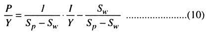
Thus, the profit share of income is given by the share of investment to income. The stability of the model is given by 0 < S_w < S_p <1. Notice that the flexibility of saving is achieved in the KM model by the assumption of different propensities to save by wage and profit earners.

The specific value of savings necessary to obtain the solution would be given by income distribution between income classes. Given S_p and S_w, l/Y will determine P/Y. If it is assumed that S_w = 0, we then obtain – P/Y = 1/S_w x 1/Y ……… (11)

Note that, if the capital-output ratio K/Y is fixed as in the HD model, we can write

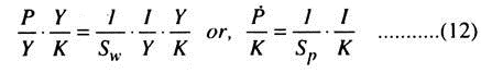
Since P/K = Y, the rate of profit .earned on capital, and I/K = J, the rate of accumulation, we have v = 1/S_p j or, S_pv = J……… (13).

This conclusion betrays remarkable affinity to the Von Neumann case, where Neumann puts S_p = 1. Thus, all profits are saved and in equilibrium we obtain V = J(=n) where n is the natural growth rate, which is assumed thus: the rate of growth is given by the rate of profit which is determined by the propensity to save of the profit earners.

Kaldor’s introduction of an ‘alternative’ theory of distribution to analyse the problem of economic growth is interesting. However, several important criticisms have been leveled at the Kaldor’s theory.

First, Pasinethi mentions a ‘logical slip’ in Kaldor’s argument when he observed that, although he has allowed workers to save, he did not allow these savings to accumulate and generate economic growth. Pasinethi has demonstrated that on a steady-state growth path the profit rate depends only on the growth rate and the propensity to save by the capitalists, it is independent of the propensity to save by the workers.

However, if it is assumed that capitalists as a class have been banished and capital is owned by the workers alone, than the relevant variables in the balanced growth path will be given by S_w and n. Second, Kaldor’s assumption about the fixed propensities to save disregards the impact of life cycle on save and work. Third, the assumption of a fixed class of income receivers is regarded as unrealistic.

Finally, Kaldor’s Model fails to exhibit an explicit behavioural mechanism, which will ensure that the actual distribution of income will be such as to maintain the steady-state growth path.