Euler’s Product Exhaustion Theorem (With Diagram)

The below mentioned article provides a close view on the Euler’s Product Exhaustion Theorem.

Euler’s theorem can be solved as under. Let С and L be the quantities of two factors of production, capital and labour respectively and P the total product of these factors. Then P = f(C, L).

In other words, if P is a linear homogeneous function (f) of С and L, the following equation will hold:

P = (Əf/ƏC) C + (Əf/ƏL) L ….. (1)

If the quantities of all inputs С and L are increased k-fold, the output P will also increase k-fold. Then the production function becomes

kP=f(kC, kL)

By taking the total derivate of kP with respect to k, we have

(dk/dk)P = Əf/ƏkC. dkC/dk + Əf/dkL. dkL/dk

Or P= (Əf/ƏkC)C + (Əf/dkL)L [By eliminating dk/dk]

P=(Əf/ƏC)C + (Əf/dL)L [k=1]

where Əf/ƏC is the marginal product of capital and Əf/ƏL is the marginal product of labour. And Əf/ƏC. С is the share of capital in the product P, and Əf/ƏL. L is the share of labour in the total product. The above equation states that the marginal product of capital (Əf/ƏC) multiplied by units of capital employed (C) plus the marginal product of labour (Əf/ƏL) multiplied by the number of labourers (L) exactly equals the total product, P. Thus total factor payments exhaust the total value of the product.

Diagrammatic Representation of Euler’s Theorem. To restate, Euler’s theorem is

It is illustrated in Figure 1 where labour is taken on the horizontal axis and the total product on the vertical axis. The curve OP is the total product curve or the production function: P = f (C, L). The tangent T on the OP curve at point G represents constant returns to scale.

The slope at point G is equal to

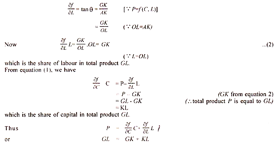
Hence the total product (GL) is fully exhausted (or distributed) between the two factors, capital (KL) and labour (GK).

Assumptions:

Euler’s theorem (or the adding up problem) is based on the following assumptions:

First, it assumes a linear homogeneous production function of first degree which implies constant returns to scale

Second, it assumes that the factors are complementary, i.e., if a variable factor increases, it increases the marginal productivity of the fixed factor.

Third, it assumes that factors of production are perfectly divisible.

Fourth, the relative shares of the factors are constant and independent of the level of the product.

Fifth, there is a stationary, riskless economy where there are no profits.

Sixth, there is perfect competition.

Last, it is applicable only in the long-run.

Explanation:

Given these assumptions, Wick-steed proved with the help of Euler’s theorem that when each factor was paid according to its marginal product, the total product would be exactly exhausted. This is based on the assumption of a linear homogeneous function.

Wick-steed did not differentiate between the laws of increasing, constant and diminishing returns. He held that under perfect competition and constant returns to scale, the product exhaustion theorem was universally valid.

Wick-steed’s solution was treated by Edge worth with mockery and Pareto objected to the assumption of constant returns to scale. Wicksell, Walras and Barone also criticised him. They pointed out that the production function does not yield a horizontal long-run average cost curve (LRAC) but a U-shaped LRAC curve. The U- shaped LRAC curve first shows decreasing returns to scale, then constant and in the end increasing returns to scale, “Where Wick-steed went wrong,” writes Hicks, “was his assumption that he could argue from the shape of the curve at one particular point to the general shape of the curve.”

Wick-sell proved that the product exhaustion problem held under perfectly competitive conditions in the long-run when profits were zero. He regarded it as a condition of equilibrium at the minimum point of firm’s long-run average cost curve (LRAC) where the linear homogeneous production function was satisfied.

Suppose an entrepreneur is left with more than the marginal product of the resource he owns after paying all other resources their marginal products. Then all owners of resources are induced to become hiring agents and in the process the difference between the total product and the rewards to factors is eliminated.

Conversely, if the residual left with the entrepreneur is less than his marginal product, after paying the other resources their marginal products, he will cease to be a producer and lend his services for its marginal product. Thus a firm under competitive conditions will produce at a level where the total product is exactly distributed according to the marginal product of the factor.

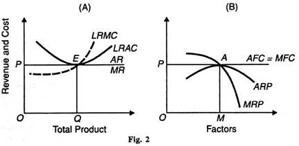
This solution of the product exhaustion theorem is based on a profitless long-run, perfectly competitive equilibrium position of a firm which operates at the minimum point, E of its LRAC curve, as shown in panel (A) of Figure 2. At this point the firm is in full equilibrium, the marginal revenue productivity (MRP) of the factors being equal to the combined marginal cost of the factors (MFC).

This is shown in panel (B) of Figure 2 where MRP = MFC at point A. It is at point A that the total product OQ is exactly distributed to OM factors and nothing is left over.

As studied above, the product exhaustion problem is solved with a linear homogeneous production function: P = (ƏP/ƏC) +C (ƏP/ƏL)L. If, however, there are diminishing returns to scale, less than the total product will be paid to the factors: P> (ƏP/ƏC) +C (ƏP/ƏL)L. In such a situation, there will be super-normal profits in the industry.

They will attract new firms into the industry. As a result, output will increase, price will fall and profits will be eliminated in the long-run. In this way, the distributive shares of the factors as determined by their marginal productivities will completely exhaust the total product.

Criticism:

In reality, constant returns to scale are incompatible with competitive equilibrium. For if long-run cost curve of the firm is horizontal and coincides with the price line the size of the firm is indeterminate; if it is below the price line the firm will become a monopoly concern; and if it is above the price line, the firm will cease to exist.

While in the case of increasing returns to scale more than the total product will be distributed, because doubling the factors wills more than double the total product. But increasing returns are incompatible with perfect competition, since the economies of production lead to the lowering of the cost of production and in the long-run there is a tendency towards the establishment of a monopoly

The whole analysis is based on the assumption that factors are fully divisible. Since the entrepreneur cannot be varied, we have not taken him as a separate factor. In fact, entrepreneurship disappears in the stationary economy.

When there is full equilibrium at the minimum point of the LH4C curve, there is no uncertainty and profits disappear altogether. So the assumption of an entrepreneur less economy is justified for the solution of the adding-up problem. But once uncertainty appears, the entrepreneur becomes a residual claimant and the exhaustion of the production problem disappears,

Under imperfect or monopolistic competition the total product adds up to more than the share paid to each factor, that is, P is greater than С and L. Taking an imperfect labour market, the average and marginal wage curve (AW and MW) slope upward and the average and marginal revenue product curves (ARP and MRP) are inverted U-shaped, as shown in Figure 3.

Equilibrium is established at point E where the MRP curve cuts the MW curve from above. The firm employs OQ units of labour by paying QA wage which is less than the marginal revenue product of labour QE. Thus workers are paid less than their marginal productivity when there is imperfect competition. This argument applies not only to labour but to all shares even under constant returns to scale in the industry.

The product exhaustion theorem, however, holds true under monopolistic competition when the firm is in equilibrium. At equilibrium, the marginal cost curve cuts the marginal revenue curve and the average revenue curve is tangent to the average cost curve.

It follows that the total outlay for factors and the total revenue product will be equal. If now a small change in factors is made, keeping their prices constant, the increase in the total revenue product is approximately proportional to the increase in the outlay for factors.

Thus if each factor included in the cost curve is paid according to its marginal revenue product at equilibrium, the total product of the firm will be exactly exhausted among them. But if there is monopoly, payment in accordance with marginal product will not exhaust the total product.