Let us make an in-depth study of the Derivation of Aggregate Demand Curve.
To start with we derive the aggregate demand curve from the IS-LM model and explain the position and the slope of the aggregate demand curve.
The aggregate demand curve shows the inverse relation between the aggregate price level and the level of national income. Now we may established this relation on the basis of the IS-LM model.
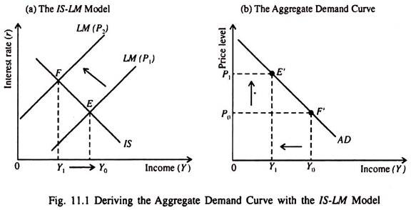
Suppose we hold the nominal money supply constant. Now if the price level (P) rises, the supply of real money balances (M/P) falls. As a result the LM curve shifts upwards to the left.
ADVERTISEMENTS:
This leads to a rise in r and a fall in Y as shown in part (a) of Fig. 11.1.
We see that as the price level rises from P0 to P1 the income level falls to from Y0 to Y1. This inverse relationship between Y and P is captured by the aggregate demand curve, as shown in part (b) of Fig. 11.1.
Thus the aggregate demand curve is a locus of points showing alternative combinations of P and Y that are consistent with the general equilibrium of the goods market and money market, i.e., equilibrium r and Y — shown by the intersection of the IS and LM curves.
ADVERTISEMENTS:
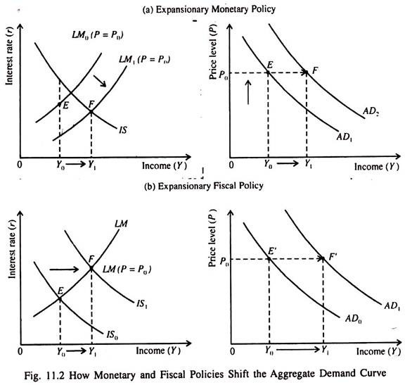
The aggregate demand curve shifts due to any event that shifts the IS curve or the LM curve (when P remains constant). For instance, if M increases Y rises if P remains constant. As a result aggregate demand curve shifts to the right as shown in part (a) of Fig. 11.2. The converse is also true. A fall in M reduces Y and shifts the aggregate demand curve to the left.
Similarly for a constant price level, an increase in G or a cut in T shifts the aggregate demand curve to the right, as shown in part (b) of Fig. 11.2. The converse is also true. A fall in G or an increase in T lowers Y or shifts the aggregate demand curve to the left.
The Economy in the Long Run:
ADVERTISEMENTS:
The basic IS-LM model is presented on the basis of the assumption that the price level remains fixed. So like the Keynesian model of income determination it is a fix-price model. And thus it shows the behaviour of the economy in the short run.
If we allow the price level to move up or down in order to ensure that the economy produces its full employment (potential) output, we can use the IS-LM model to describe the behaviour of the economy in the long run. Recall that the full employment level of output is also called the natural rate of output which is consistent with the natural rate of unemployment.
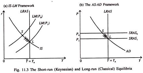
In Fig. 11.3 the LM curve is drawn for a fixed price level, P0. The short-run equilibrium of the economy is at point S, where the IS curve intersects the LM curve. This is short-run equilibrium of the Keynesian type because it is a situation of underemployment equilibrium.
At point S the economy’s output (income) is less than its natural rate. In Fig. 11.3(b) we see that at the price level P0, the quantity of output is below the natural rate. As in the Keynesian model, the aggregate demand for goods and services is not adequate to permit the economy turn out its potential output.
In both diagrams point S indicates short-run equilibrium because the price level remains fixed at P0. However, such a situation cannot persist for long. Sooner or later prices have to fall due to the persistence of demand deficiency. Price flexibility does the trick here. The economy ultimately moves back to its natural rate.
As soon as the price level falls to P1 the economy reaches its long-run equilibrium, at point L. Fig. 11.3(b) shows that at point L, aggregate demand equals the full employment (potential) output. In Fig. 11.3(a) the same long-run equilibrium is achieved by shifting the LM curve to the right. The LM curve shifts due to the fall in P1 which, in its turn, increases real money balances (M/P).
In both the figures point S is the Keynesian equilibrium where P remains fixed. This point shows that output deviates from its natural rate. In contrast L is the classical equilibrium. In this case price flexibility ensures automatic full employment, (i.e., the economy always produces at the natural rate.)
The Keynesian model is based on the assumption that the price level remains fixed. So output adjusts in response to changes in aggregate level demand for goods and services.
ADVERTISEMENTS:
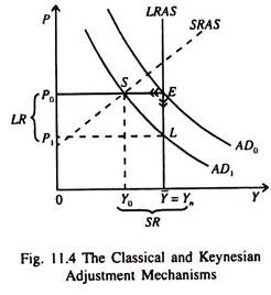
In contrast the classical model is based on the assumption that output remains fixed at the full employment level and price adjusts in response to changes in aggregate demand. The comparison is shown in Fig. 11.4. If the aggregate demand curve shifts to the left, in the short run output falls to Y0, price remaining the same at P0. But in the long run price P0 to P1 output remaining the falls from same.
Thus in the short run the price level remains fixed and output adjusts. This is the Keynesian adjustment mechanism. In the long run the economy moves from point E to L.


