Top 3 Techniques of Demand Forecasting | Products | Economics

The following points highlight the top three techniques of demand forecasting. The techniques include: 1. Survey Methods 2. Opinion Poll Methods 3. Statistical Methods.

1. Survey Methods:

Under survey methods surveys are conducted about the consumers’ intentions, opinions of experts, survey of managerial plans, or of markets. Data obtained through these methods are analyzed, and forecasts on demand are made. These methods are generally used to make short-run forecast of demand.

Consumers’ Survey:

Consumers’ survey method of demand forecasting involves direct interview of the potential consumers. Consumers are simply contacted by the interviewer and asked how much they would be willing to purchase of a given product at a number of alternative product price levels.

Consumers’ survey may take any form as:

a. Complete Enumeration

b. Sample Survey, or

c. End-Use Method

a. Complete Enumeration Method:

In complete enumeration survey, all the consumers of the product are contacted and asked to indicate their plans to purchasing the production in question for the forecast period.

The demand forecast for the’ total census consumption is obtained simply by adding the intended demand of all consumers as:

DF = Id₁ + ID₂ +……….. ID_n …(2.1)

Where,

DF = demand forecast for all consumers

ID₁ = intended demand of consumer 1.

ID₂ = intended demand of consumer 2.

The probable demand of all the consumers are summed up to obtain the sales forecast. This method facilitates the collection of firsthand information and is free from bias. The method has its share of disadvantages too. This method can be applied in case of those products only whose consumers are located in a certain region. If the consumers of the product are widely dispersed, this method proves to be costly and time consuming. Demand estimation through this method may not be reliable because consumers have not thought out in advance what they would do in these hypothetical situations.

Also:

(i) Consumers may not be aware of their exact demand and hence may not be able or willing to answer the questions;

(ii) The consumers may give hypothetical answers to hypothetical questions;

(iii) Their responses may be biased according to their own expectations about the market conditions;

(iv) Their plans may get altered with alterations in the factors not included in the questionnaire, and

(v) When we get to the effects of advertising on demand, the problems of such a direct interview approach becomes even more appeared.

b. Sample Survey Method:

Useful data for forecasting demand can also be obtained from surveys of consumer plans. Unlike the complete enumeration method, under the sample survey method, only a few potential consumers from the relevant market selected through an appropriate sampling method, are interviewed. The survey may be conducted either through direct-interview or mailed questionnaire to the sample consumers.

The total demand may be forecast with the help of following formula:

Where,

N the population of consumers

n sample surveyed.

Then the probable demand expressed by each selected unit is summed up to get the total demand for the forecast period. Total sample demand is then multiplied by the ratio of number of consuming units in the population to the number of consuming units in the sample. If the sample selected is adequately representative of the population, the results of the sample are more likely to be similar with the results of the population. This method is simpler, economical and time- saving as compared to the complete enumeration survey.

Although surveys of consumer demand can provide useful data for forecasting, their value is highly dependent on the skills of their originators. Meaningful surveys require careful attention to each phase of the process. Questions must be precisely worded to avoid ambiguity. The survey sample must be properly selected so that responses will be representative of all customers. Finally, the methods of survey administration should produce a high response rate and avoid biasing the answers of those surveyed. Poorly phrased questions or a nonrandom sample may result in data that are of little value.

Even the most carefully designed surveys do not always predict consumer demand with great accuracy. In some cases, respondents do not have enough information to determine if they would purchase a product. In other situations, those surveyed may be pressed for time and be unwilling to devote much thought to their answers.

Sometimes the response may reflect a desire (either conscious or unconscious) to put oneself in a favorable light or to gain approval from those conducting the survey. Because of these limitations, forecasts seldom rely entirely on results of consumer surveys. Rather, these data are considered supplemental sources of information for decision- making.

c. End-Use Method:

The end-use method of demand forecasting has considerable amount of both theoretical and practical values. This method involves a survey of firms in all industries using the product and projects the sale of the product under consideration based on demand survey of the industries using this product as an intermediate product. Demand for the final product is the end-use demand of the intermediate product used in the production of this final product.

The end-use method of demand forecasting consists of four distinct stages of estimation:

(1) Obtain the information about the potential uses of the product in question.

(2) Determine suitable technical ‘norms’ of consumption for each and every use of the product under study.

(3) For the application of the norms, it is necessary to know the desired or targeted levels of output of the individual industries for the reference year and also the likely development in other economic activities which use the product and the likely output targets.

(4) Finally, the product-wise content of the item for which the demand is to be forecast, is aggregated which gives the estimate of demand for the product as a whole for the terminal year in question.

Thus, end-use demand estimation of an intermediate product may involve many final goods industries using this product at home and abroad. Once the demand for final consumption goods including their export net of imports is known, the demand for the product used as intermediate good in the production of these final consumption goods with the help of input-output coefficients can be estimated. The input-output tables containing input-output coefficients for particular periods are made available in every country either by the government or by research organizations.

Except in the case of intermediate products, demand forecasting through end-use method is neither desirable nor feasible. Further, as the number of end-users of a product increases it becomes more and more inconvenient to use this method. This method is quite useful for industries that are largely producers’ goods, like aluminium.

Making forecasts by this method requires building up a schedule of probable aggregate demand for inputs in future by consuming industries and various sectors. In this method, technological, structural and other changes, which might influence the demand, are taken care of in the very process of estimation. This aspect of the end- use approach is of particular importance.

Advantages of End-Use Method:

(1) It helps to estimate the future demand for an industrial product in considerable detail by types and size. By probing into the present use-pattern of consumption of the product, the end use approach affords every opportunity to determine the types, categories and sizes likely to be demanded in future.

(2) The method assists to trace and pinpoint at any time in future as to where and why the actual consumption has deviated from the estimated demand. Suitable revisions can also be made from time to time based on such examination.

2. Opinion Poll Methods:

The opinion poll methods make demand estimation by using opinions of those who possess knowledge of the market, such as professional marketing experts and consultants, sales representatives and executives. The collective judgment of knowledgeable persons can be an important source of information.

In fact, some forecasts are made almost entirely on the basis of personal insights of key decision makers. This process may involve managers conferring to develop projections based on their assessment of economic conditions facing the firm. In other circumstances, the company’s sales personnel may be asked to evaluate future prospects. In still other cases, consultants may be employed to develop forecasts based on their knowledge of the industry.

These methods include:

i. Experts’ Opinion:

The researcher identifies the experts on the commodity whose demand forecast is being attempted, and probes with them on the likely demand for the product in the forecast period. This method consists of securing views of the salesmen and/ or sales management personnel. There are many variations.

The combined view of the sales force as to future sales expectations may be secured by carefully scrutinizing at successive executive levels and future sales estimates submitted by the salesmen individually. Another method would be to rely only on the specialized knowledge of the company’s sales executives in preparing sales forecasts.

The advantages of this method consist of:

(a) This method makes use of specialized knowledge of persons closest to the market;

(b) Provides sales force with greater confidence in getting sales quotas developed;

(c) Greater stability through magnitude of sample;

(d) Placing of responsibility for the forecasts on those who are expected to produce results.

The disadvantages advanced are that:

(a) Salesmen are poor estimators being unduly optimistic;

(b) Salesmen are often unaware of the broad economic patterns and cannot forecast long-term trends;

(c) The sales force’s time is in this way curtailed for the primary job of selling; and;

(d) Salesmen may intentionally understate the demand if quotas are set on the basis of this information.

ii. Delphi Method:

The Delphi method is a facilitated process of gaining consensus within a group of anonymous participants. The facilitator sends a forecast questionnaire to each member of the Delphi group. Anonymity is critical in this method to prevent a few group members from dominating the decision. When the questionnaire is returned, the responses are statistically summarized and then sent back out to the group. Each Delphi member has the choice to modify their previous responses based on the responses of the group. This is a reiterative process that continues until a consensus is obtained.

The Delphi method is used for new products or for very long-range forecasts. However, it is a time-consuming process that is highly dependent on the quality of the questionnaires. Further, participants may provide inadequate responses because there is no accountability.

Under Delphi method opinions are collected from experts and efforts are made to match them. This is done by bringing the experts together, arranging meetings and arriving at some narrow range for the forecast under attempt to give the interval forecast directly and for arriving at a point forecast by tampering it with the overall assessment of the researcher or the coordinator of the forecasting exercise.

Generally, the forecast proceeds through the following stages:

(i) Request is made to all the experts of product to give their individual estimates for the likely demand.

(ii) If the difference in forecasts is significant, the experts are invited for a conference on the subject, present the problem with regard to differences in their estimates. By arguing, convincing others and getting convinced, exchanging views with colleagues, efforts are made to narrow the limits for likely demand.

(iii) If the range of variations is still large the exercise continues till the coordinator is able to arrive at an acceptable range.

(iv) Declare the so arrived range as the interval demand forecast for the product for the period for which it is done.

(v) Take a simple average of the lower and upper values of the forecast and declare the point forecast for the variable under forecasting.

The use of Delphi technique can be illustrated by a simple example. Suppose that a panel of six outside experts is asked to forecast a firm’s sales for the next year. Working independently, two panel members forecast an 8 percent increase, three members predict a 5 percent increase, and one person predicts no increase in sales. Based on the responses of the other individuals, each expert is then asked to make a revised sales forecast. Some of those expecting to rapid sales growth may, based on the judgments of their peers, present less optimistic forecasts in the second iteration.

Conversely, some of those predicting slow growth may adjust their responses upward. However, there may also be some panel members who decide that no adjustment of their initial forecast is warranted. Assume that a second set of predictions by the panel includes one estimate of a 2 percent sales increase, one of 5 percent, two of 6 percent, and two of 7 percent.

The experts again are shown each other’s responses and asked to consider their forecasts further. This process continues until a consensus is reached or until further iterations generate little or no change in sales estimates. Delphi method is quite sound but it could be tedious and costly.

In the situations where the number of experts is not too large and they are co-cooperative, and the researcher has the necessary fund and the authority to perform the task, the Delphi method could be appropriate for demand forecasting.

The value of the Delphi technique is that it aids individual panel members in assessing their forecasts. Implicitly, they are forced to consider why their judgment differs from that of other experts. Ideally, this evaluation process should generate more precise forecasts with each iteration. The usefulness of expert opinion depends on the skill and insight of the experts employed to make predictions.

One problem with the Delphi method can be its expense. Frequently, the most knowledgeable people in an industry are in a position to command large fees for their work as consultants. They may be employed by the firm, but have other important responsibilities, which means that there can be a significant opportunity cost in involving them in the planning process.

Moreover, experts are unwilling to be influenced by the predictions of others on the panel. Although predictions by experts are not always the product of “hard data,” their usefulness should not be underestimated. Indeed, the insights of those closely connected with an industry can be of great value in forecasting

iii. Surveys of Managerial Plans:

Surveys of managerial plans can be an important source of data for forecasting. The rationale for conducting such surveys is that plans generally form the basis for future actions. For example, capital expenditure budgets for large corporations are usually planned well in advance. Thus a survey of investment plans by such corporations should provide a reasonably accurate forecast of future demand for capital goods.

iv. Market Experiments:

Market experiments (actual or simulated) are performed to generate demand forecasts. A potential problem with survey method is that survey responses may not translate into actual consumer behavior. Consumers do not necessarily do what they say they are going to do. This weakness can partially be overcome by use of market experiments designed to generate data prior to the full-scale introduction of a product or implementation of a policy.

Market experiment can be performed in two forms:

(a) Test Market:

In order to set a market experiment the firm first selects a test market that may consist of several cities, a region of the country, or a sample of consumers taken from a mailing list. The experiment may incorporate a number of features such as evaluating consumer perception of a new product in the test market. In other cases, different prices for an existing product might be set in various cities in order to determine demand elasticity. A third possibility would be a test of consumer reaction to a new advertising campaign.

There are several factors that managers should consider in selecting a test market. The location should be of manageable size. If the area is too large it may be expensive and difficult to conduct the experiment and to analyze the data. Second, the residents of the test market should be representative of the overall population of the United States in age, education, and income otherwise the results may not be applicable to other areas. Finally, it should be possible to purchase advertising that is directed only to those who are being tested.

(b) Laboratory Tests:

Another way of conducting market experiment is consumer clinic or controlled laboratory experiment. Here, consumers are given some money to buy in a stipulated store goods with varying prices, packages, displays etc. and consumers’ responsiveness to these variations are studied. Thus the laboratory experiment yields the same results as the field market experiment.

Market experiments have an advantage over surveys in that they reflect actual consumer behavior, but they still have limitations. One problem is the risk involved. In test markets where prices are increased, consumers may switch to products of competitors. Once the experiment has ended and the price reduced to its original level, it may be difficult to regain those customers.

Another problem is that the firm cannot control all the factors that affect demand. The results of some market experiments can be influenced by bad weather, changing economic conditions, or the tactics of competitors. Finally, because most experiments are of relatively short duration, consumers may not be completely aware of pricing or advertising changes. Thus their responses may understate the probable impact of those changes.

Limitations:

The market experiment methods have certain serious limitations that reduce the reliability of the method considerably:

i. Experimental methods are very expensive so small firms cannot afford them. Being a costly affair, experiments are usually carried out on a scale too small to permit generalization with a high degree of reliability.

ii. Experimental methods are based on short-term and controlled conditions that may not exist in an uncontrolled market. Hence the results may not be applicable to the uncontrollable long-term conditions of the market.

iii. Changes in socio-economic conditions taking place during the field experiments, such as local strikes or lay-offs, advertising program by competitors, political changes, natural calamities, may invalidate the results. Tinkering with price increases may cause a permanent loss of customers to competitive brands that might have been tried.

Despite these limitations, however, market experiment method is often used to provide an alternative estimate of demand, and also as a check on results obtained from statistical studies. Besides, this method generates elasticity coefficients which are necessary for statistical analysis of demand relationships.

3. Statistical Methods:

We have discussed survey and experimental methods of demand forecasting. These methods are more appropriate estimating demand for a product for the short term.

In this section statistical methods that depend upon time-series and cross-section data and are appropriate for long term demand forecasting have been discussed:

The following are the main statistical methods:

i. Trend Projection Methods

ii. Barometric Methods, and

iii. Econometric Methods

i. Trend Projection Methods:

Trend projection is one of the most widely used techniques of demand forecasting. A trend in time-series of a variable is the long- term change in it? This method requires a long and reliable time series data. This method assumes that the factors responsible for the past trends in the variable to be projected will continue to play their part in future in the same manner and to the same extent as they did in the past in determining and magnitude and direction of the variable. There can be linear or non­linear trends in demand for a product.

Mostly, linear trends and constant rate of growth trend are used to predict future demand. These methods dispense with the need for costly market research because the necessary information is often already available with the company. Since the method does not reveal cause and effect relationship, it has been considered as a ‘naive approach’.

Despite, “There is nothing uncomplimentary in the adoption of such an approach. It merely represents one of the several means to obtain an insight of what the future may possibly be and whether or not the projections made using these means are considered as most appropriate will depend very much on the reliability of past data and on the judgment that is to be exercised in the ultimate analysis.”

For forecasting demand through trend projection methods the time series data on sales is required. In case of well- established firms with long business history, such data is available in sales records. New firms can obtain necessary data from the existing firms belonging to the same industry.

Three important techniques of trend projection based on time-series data are described below:

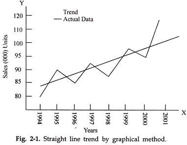
(i) Graphical, Inspection or Freehand Method:

Under this method a graph of historical data on the variable under forecasting is drawn, it is then extrapolated visually up to the forecast period, and finally the value of the variable in the forecast period is read out from the graph to yield the requisite forecast.

In Fig.2.1 sales in thousand units is shown on Y-axis and the time starting from 1994 to 2001 is shown on X-axis. The sales data is plotted on the graph and the plotted points are joined through a line. Then a line with minimum distance from the points is drawn. By extending the trend line we may forecast an approximate sale for the year 2005 or 2007.

Though this method is simple and economical, yet the forecasts obtained suffer from subjectivity and personal bias of the analyst in the extrapolation of the curve. However, since historical data of no variable when plotted usually lie on any smooth curve extrapolation would never be unique and the method would always suffer from subjectivity.

The graphical technique is explained with the help of following illustration:

Illustration:

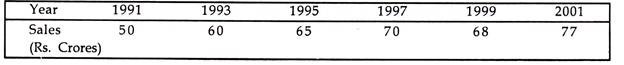
Using the free hand or graphic method, fit a straight line trend to the following time series data on sales of a company.

Choosing a suitable scale, years are marked along the x-axis and corresponding sales values are marked along the y-axis. The points so obtained are then joined by straight line that shows the behavior of sale values over the given period. Then we draw a free hand straight line through the points of actual data for smoothing the time series data obtain the trend. The behavior of actual data and the trend line are shown in Fig.2.1.

(ii) Trend Fitting or Least Square Method:

Under this method, extrapolation of historical data is attempted through estimation of alternative trend equations.

A trend equation is one in which the variable under forecast is made simply as a function of time:

This technique uses statistical formulae to find the trend line which ‘best fits’ the available data.’ The trend line is the estimating equation which can be used for forecasting demand by extrapolating the line for future and reading the corresponding values of sales on the graph.

Linear Trend:

The estimating linear trend equation of sales is written as:

Sales = a + b (year number)

Or S = a + bT .… …(2.3)

where, a and b are calculated from past data and

T is the year number for which the forecast is required.

The following illustration explains how demand forecasting is done with the help of Least Square Method.

Illustration:

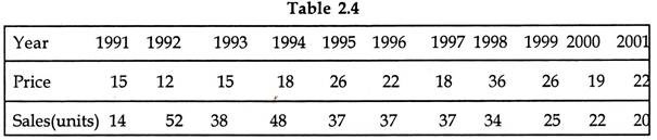
The sales records of a hypothetical company reveal the following data

Estimate sales for the years 2003 and 2005.

Solution- To find the values of a and b in the trend equation S = a + b

we will need to solve the two normal equations, viz.

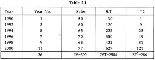
Substituting the above values in the two normal equations, we get

270 = 6a + 36b

1,784 = 30a + 286b

Solving these equations for a and b, we get.

a = 1.53 and

b = 6.8.

Thus the trend equation becomes S = 1.53 + 6.8T.

Years 2003 and 2005 take on the year numbers 14 and 16. By substituting these values for T. we get the sales for these years as Rs. 96.73 crores and Rs. 110.33 crores respectively.

The trend method is basically an objective method. The trend equation given above assumes that there is a linear (or proportional) change in sales over time. In fact, the trend equation can take a linear or a non-linear form.

Non-Linear Trend:

Many time series data concerning with business and economic activities showing constant initial growth and not approaching certain upper limit can best be described by exponential function.

The exponential form of equation may be of the following forms:

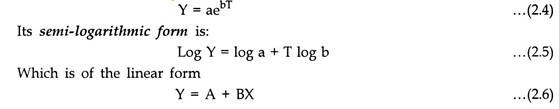
Now we can apply the usual procedure of fitting the linear trend. Finally, the values of a and b can be determined by taking antilogarithms of a and b respectively, i.e.,

a = antilog a and b = antilog b

Putting these estimated values of a and b in equation (2.4). we get the required exponential trend.

Illustration:

The profits of a concern for five years ending 2001:

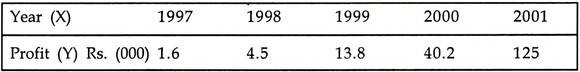
Find the trend values for the year 1997 – 2001 using an equation of the form

Y = ab^X

Solution:

The equation to be fitted is Y = ab^X

or Log Y = log a + T log b

y = A + BX

where Y = log Y, A= log a and B = log b

The values of a and b can be obtained from the following normal equations:

Sy = Na + bS X

SXy=aSX+bSX² …(2.7)

Fitting of Exponential Trend:

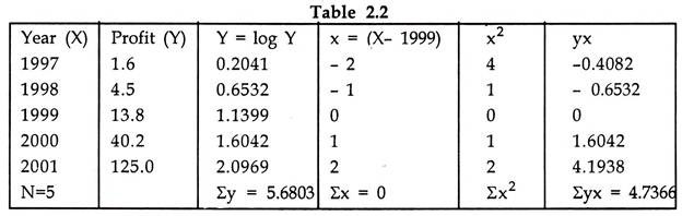
Putting the values from the table in 2.2

5.06803 = 6A A = 1.1397 a = antilog (1.1397) = 13.79

4.7366 = 10A B = 0.4737 b = antilog (0.4737) = 2.977

Putting the values of a and b in (2.2), the fitted trend is

Y = (13.79) (2.997)^x, where X = (x – 1999)

For computation of trend values, we make use of equation 2.6

y = 1.1397 + 0.4737 X

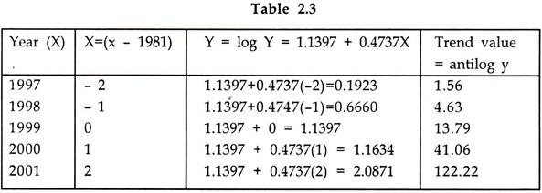
Thus in the above table the trend values from 1997 to 2001 have been computed. Double-log trend of the form.

The double log trend of equation is used when growth rate is increasing.

The equation is written as:

Y = aT^b … (2.8)

Or its double logarithmic form

Log Y = log a + b log T … (2.9)

Polynomial trend of the form

Y = a + bT + cT² … (2.10)

In these equation Y is variable (may be sales), T is time, a, b and c are constants and e = 2.718. Once the parameters of the equation are estimated, it becomes easy to forecast demand for the time to come.

We can similarly build up trend equations for polynomials of degrees higher than three, but they are seldom used in business forecasting in practice. In case of the second-degree polynomial trend, the slope dS/dT changes direction (from positive to negative, or vice versa) only once. Similarly in the case of the third degree polynomial trend, the slope changes direction only twice.

Selection of the best trend line out of the various linear and non-linear trend equations depends upon the theoretical considerations and empirical suitability. Once the decision is taken regarding the most appropriate equation for a given sales data the forecast can be made by fitting the equation to the data.

(iii) Exponential Smoothing:

If the variable under forecast does not follow any specific trend, the trend method is inappropriate. The smoothing method would be more useful. There are versions of the smoothing method- simple smoothing (averaging) and weighted smoothing. One characteristic of this method is that each observation has the equal weight.

In the simple smoothing, a simple average of the specific number of observations (called the ‘order’) is taken, while in the latter, a weighted average is taken out. Since, more recent observations will contain more accurate, information about the future than those at the beginning of the series for estimating the future, the weighted is preferred to the simple smoothing and the weights are assigned in a descending order as one goes from the current observations to the past ones. For example, the sales history of the last three months may be more relevant in forecasting future sales than data for sales ten years in the past.

Exponential smoothing is a technique of time-series forecasting that gives greater weight to more recent observations.

The first step is to choose a smoothing constant, ± , where 0 < ± < 1.0.

If there are n observations in a time series, the forecast for the next period n+1 is calculated as a weighted average of the observed value of the series at period n and the forecasted value for that same period.

The formula for weighted average may be written as:

Where,

F_n+1 is the forecast value for the next period,

X_n is the observed value for the last observation, and

F_n is a forecast of the value for the last period in the time series.

The forecast values for F and all the earlier periods are calculated in the same manner. Specifically,

For second observation t= 2 and going to the last.

The exponential smoothing constant chosen determines the weight given to different observations in the time series. As ± approaches 1.0, more recent observations are given greater weight. For example, if ± = 1.0, then (1- ±) =0. In contrast, lower values for ± give greater weight to observations from previous periods.

For example, if a firm’s sales over the last ten weeks are given below:

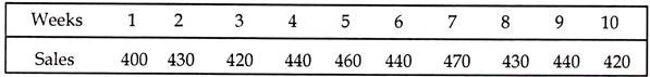
Assuming F₂ = F₁ = X₁. If ± = 0.20, then

F₃ = 0.20 (430) + 0.80 (400) = 406.0 and

F₄= 0.20 (420) + 0.80 (406) = 408.8

The forecasted values for different values of ± may be calculated.

It should be noted that the smoothed data show much less fluctuation than the original sales data. Note also that as ± increases, the fluctuations in the F increase, because the forecasts give more weight to the last observed value in the time series.

Any value of ± may be used as the smoothing constant. The criteria for selecting the constant might be the analyst’s intuitive judgment regarding the weight that should be given to more recent data points. But there is also an empirical basis for selecting the value of ±.

Thus, the method of exponential smoothing allows more recent data to be given greater weight in analyzing time-series data. Also as additional observations become available, it is easy to update the forecasts. There is no need to re-estimate the equations, as would be required with trend equation. However, this method does not provide very accurate forecasts if there is a significant trend in the data. If the time trend is positive, forecasts based on exponential smoothing will likely be too low, while a negative time trend will result in too high estimates. Simple exponential smoothing works best when there is no discernable time trend in the data.

ii. Barometric Forecasting:

Trend projection and exponential smoothing use time series data for forecasting the future. In the absence of a clear pattern in a time series, the data are of no avail for forecasting. An alternative approach is to find a second series of data that is correlated with the first. A time-series that is correlated with another time-series is called an indicator of the second series. As meteorologists use barometer to forecast weather, economists use economic indicators as a barometer to forecast trends in business activities.

Barometric method of forecasting was first developed and used in the 1920s by the Harvard Economic Service, failed to predict the Great Depression of the 1930s, but revived, refined and developed further in the late 1930s in the US by the National Bureau of Economic Research (NBER). Initially, the technique was developed to forecast the general trend in overall economic activities, but it can be applied to forecast prospects of demand for a product. The technique identifies relevant economic indicators on the movement of which future trends are forecast.

The barometric forecasting technique identifies the relevant economic indicators, constructs an index of these indicators and observing movements of the index forecasts future trends.

Two techniques are discussed for barometric forecasting:

1. Leading Indicators, and

2. Composite and Diffusion Indices

1. Leading Indicators Method:

This method involves three steps:

i. Identification of the leading indicator for the variable under forecasting.

ii. Estimation of the relationship between the variable under forecasting and its leading indicator.

iii. Derivation of forecasts

Three types of economic indicators are identified for constructing the index:

a. Leading Indicators,

b. Co-Incidental Indicators

c. Lagging Indicators.

a. Leading Indicators:

If changes in one series consistently occur prior to changes in another series, a leading indicator has been identified. The leading indicators move up or down ahead of some other indicators. Leading indicators are of primary interest for the purposes of forecasting.

As a meteorologist makes use of changes in barometric pressure for weather forecast, leading indicators can be used to predict variations in general economic conditions. Movement in the capital formation, new orders for durable goods, new building permits, corporate profits after tax, index of the prices of input, change in the value of inventories, requests for loans from financial institutions and change in bank rate are examples of leading indicators.

b. Co-Incidental Indicators:

If two data series increase or decrease at the same time, one series may be regarded as a coincident indicator of the other series. In other words, the co-incidental economic indicators move up or down simultaneously with the level of economic activity.

Gross national product at constant prices, rate of employment, sales by different sectors, the rates at which commercial banks accept deposits from and lend to the private sector are more or less the coincident series with regard to the Bank rate, rate of employment in non-agricultural sectors are the examples of co-incidental series.

c. Lagging Indicators:

The lagging indicators follow a change after some time lag. NBER identified some of the lagging indices such as rate for short-term loans, outstanding loans, labour cost per unit of manufactured output and the rate at which private money lenders accept deposits and lend to individuals is lagging series with reference to both the Bank rate and commercial banks’ deposit and lending rates.

It is not that for every variable there is a leading variable but for some they do exist. Thus, through this kind of search, one may be able to find an appropriate leading variable for the variable. If no such variable is available, this method of forecasting is also not available. Leading indicators can be used as inputs for forecasting aggregate economic variables such as GNP, aggregate consumers’ expenditure, aggregate capital expenditure, etc.

The value of leading indicators method depends on the accuracy of the indicator, adequacy and constancy of lead- time, the reason as to why one series predicts another and the cost and time necessary for data collection

2. Diffusion Indices:

The construction of an index improves the barometric forecasting. Such indices represent a single time series made up of a number of individual leading indicators. The purpose of combining the data is to smooth out the random fluctuations in each individual series and the resulting index provides more accurate forecasts.

The index is a measure of the proportion of the individual times series that increase from one month to the next. For example, if eight of the indicators increased from June to July, the diffusion index for July would be 8/11 or 72.7 percent. When the index is over 50 percent for several months, it can be forecast that economic conditions have begun to improve. As the index approaches 100 percent, the likelihood of improvement increases. On the other hand, if less than 50 percent of the indicators exhibit an increase, a downturn is indicated.

However, the technique suffers from several weaknesses:

a. The prediction record of this technique is far from perfect.

b. On several occasions indices have forecast recessions that have not occurred. The lead- time also varies from variable to variable.

c. While this approach signals the likely direction of changes in economic conditions, it says little about the magnitude of such change. As such it provides only a qualitative forecast.

d. Also strenuous efforts have been made to identify indicators of general economic conditions the managers of individual firms may find it difficult to identify leading indicators that provide accurate forecasts for their specific needs.

Despite these limitations, the use of indices improves the accuracy of barometric forecasting.

iii. Econometric Methods:

The most popular method of demand estimation among economists is perhaps the regression method that employs both the principles of economic theory and appropriate statistical methods of estimation. It requires historical data (time series and/or cross section) on the variable under forecasting and its determinants.

In other words regression analysis denotes methods by which the relationship between quantity demanded and one or more independent variables (like income, price of the commodity, prices of related goods, advertisement expenditure) is estimated. It includes measurement of error that is inherent in the estimation process.

This method involves four steps:

(a) Identification of the variables that influence the demand for the good whose function is under estimation.

(b) Collection of historical/cross section data on all the relevant variables.

(c) Choosing an appropriate form for the function.

(d) Estimation of the function.

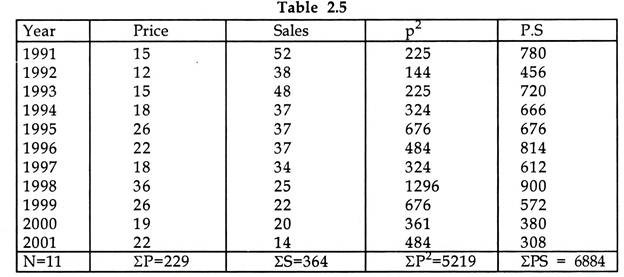
(i) Simple Linear Regression:

Simple regression analysis is used when the quantity demanded is estimated a function of a single independent variable such as price. In case of linear trend in the dependent variable, we can fit a straight line to the data, whose general form would be, for example,

Sales = a + b. Price

Fitting of the straight -line regression equation can be done either graphically or by least squares method.

In the least squares method of estimating regression line,

S = a + b.P, … (2.13)

We have to find the values of the constants, a and b by solving the two linear equations:

SS= na + Sb P

SPS = SPa+ bS P² … (2.14)

The table 4.4 provides sales data at different price levels for a hypothetical company:

Substituting the values of in the two least square equations, and solving the equations we get the values of terms a and b.

a=64.94

b=1.53

The regression equation can therefore be written as

S= 64.94 +1.53 P … (2.16)

If we assign the values to P, we can get the corresponding estimated sales.

(ii) Multivariate Regression:

Multiple linear regression generates a forecast by linking two or more independent variables to the demand for a product. For example, sales of ice cream may be dependent on the price that is charged for the product, the temperature, and the number of hours of daylight. A model would be developed which described this relationship. Given a specific price, a temperature, and a number of daylight hours, a demand forecast for ice cream will be generated.

Estimation of the parameters of an equation with more than one independent variable is called multiple regressions. In principle, the concept of estimation with multiple regression is the same as with simple linear regression, but the necessary computations can be much more complicated. For an equation with three or more independent variables, the time required to calculate the values and likelihood of an arithmetic error make manual computation impractical. Consequently, virtually all regression analysis involving multivariate equations uses computers.

Because most economic relationships involve more than a simple relationship between a dependent and a single independent variable, multiple regression techniques are widely used in economics. For example, the demand for a product usually depends on more than just the price of the good. Other variables, such as income and prices of other goods can also have an influence.

Thus, a simple regression equation involving only quantity and price would be incomplete and probably would result in an incorrect estimation of the relationship between quantity and price. This is because the effects of other variables omitted from the equation are not taken into account. Similarly, a regression equation that included only the rate of output as the determinant of costs could generate inaccurate results because other factors, such as input prices, also affect costs.

With multiple regression, it is important that the user understands how to interpret the estimated coefficients of the equation. For example, it is assumed that costs are a function of output and price of labor. Thus the multiple regression equation can be written as:

Y = A + bX + cZ , … (2.17)

Where Y is the total cost

X is output,

Z is the price of labor

a, b, c, are the coefficients to be estimated.

The coefficients of X and Z indicate the effect on total cost of a one-unit change in each variable, holding the influence of the other variable constant. For example, b shows the change in total costs for a one-unit change in output, assuming that the price of labor stays the same. The coefficient of Z estimates the effect of a unit change in labor price, assuming that the rate of output is unchanged.

The multi-variable regression equation is used where demand for a commodity is deemed to be the function of many variables or in cases in which number of explanatory variables is greater than one.

The procedure of multiple regression analysis may be described as follows:

i. Specify the independent variables that are supposed to explain the variations in the dependent variable. For example the demand for the product will be explained by the variables that are generally taken to be the determinants of demand viz., price of the product, prices of related good, consumer’s income and their tastes and preference.

For estimating the demand for durable consumer goods, (e.g. refrigerators, house, scooters), the other variables which are considered are availability of credit and prevailing rate of interest. For estimating demand for capital goods, the relevant variables are additional corporate investment, rate of depreciation, cost of capital goods, cost of other inputs, market rate of interest etc. These variables are treated as independent variables.

ii. The second step is to collect time-series data on the independent variables.

iii. Specify the form of equation that can appropriately describe the nature and extent of relationship between the dependent and independent variables.

iv. The final step is to estimate the parameters in the chosen equations with the help of statistical techniques.

The form of equation and the degree of consistency of the explanatory variable in the estimated demand function determines the reliability of the demand. The greater the degree of consistency, the higher is the reliability of the estimated demand and vice versa.

Linear Function:

When the relationship between demand and its determinants is’ linear the most common form of equation for estimating demand is as follows:

Dx = a + bPx + cPy + dY+ jA … (2.18)

where Dx = quantity demanded of commodity x; P= price of commodity X, Y= consumer’s income; P= price of the substitute; A= advertisement expenditure; a is constant (the intercept), and b, c, d, and j are the parameters expressing the relationship between demand and Px, , Py ,Y and A respectively.

In a linear function, quantity demanded changes at a constant rate with respect to change in independent variables Px, Y, Py and A. The regression coefficients are estimated by using the least square method and then, the demand can be easily forecast.

Simultaneous Equations:

The simultaneous equations method, also called the complete system approach to forecasting, is the most sophisticated econometric method of forecasting. It involves specification of a number of economic relations, one each for behavioral variable- estimation and solution of which yield the forecasting equations similar to the estimated regression equation.

One outstanding advantage of this method is that in this method we estimate the future values only predetermined variables, unlike regression equation where the value of both exogenous and endogenous variables have to be predicted. The method suffers from the demerit of complexity.