How would you Derive the Industry Demand Curve for Labour?

The following article will guide you about how would you derive the industry demand curve for labour.

The Physical Component of MRP:

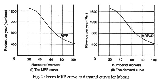
As the quantity of labour hired varies, output will vary. The hypothesis of diminishing returns, predicts what will happen: as the firm adds further units of labour to a given quantity of the fixed input, capital, the additions to output will eventually get smaller. In other words, labour’s marginal physical product declines. This is illustrated in part (i) of Figure 4. The negative slope of the MPP curve reflects the operation of the law of diminishing returns: each unit of labour adds less to total output than the previous unit.

The Value Component of MRP:

To convert the marginal physical product curve of Figure 1(i) into a curve showing the marginal revenue product of labour, we need to know the value of the extra physical product. As long as the firm sells its output in a competitive market, this value is simply the marginal physical product multiplied by the market price at which the firm sells its product.

This operation is illustrated in part (ii) of Figure 4, which shows a marginal revenue product curve for labour on the assumption that the firm sells its product in a competitive market at a price of Re. 1 per unit. This curve shows how much would be added to revenue by employing one more unit of labour at each level of total employment.

Each additional unit of labour employed adds a certain amount to total product [part (i)] and hence a certain amount to total revenue [part (ii)] and his determines the amount of labour firms will demand at each price Part (i) assumes data that are consistent with marginal productivity theory; it shows the addition to the firm’s output produced by additional units of labour hired. The curve is negatively sloped because of the law of dimin­ishing returns.

Part (ii) shows the addition to the firm’s revenue caused by the employ­ment of each additional unit of labour. It is the marginal physical product form part (i) multiplied by the price at which that product is sold. In this case the price assumed to be Rs. 1. (The multiplication is by market price because the firm is assumed to be a price taker in the market for its output.)

Since the firm equated the price of the variable input, which is labour in case, to the input’s marginal revenue product, it follows that the MRP curve, in part (ii), is also the demand curve for labour, showing how much will be employed at each price.

The basic principle is that firms should equate the addition to cost of buying another unit of a variable input with the addition to revenue caused by selling the output of that unit, which we call the input’s MRP and a value component, which is the marginal revenue of selling those extra physical units of output. Because, for simplicity, our firms are assumed to be price takers in their output markets, the marginal revenue is just the price that they face in the market.

If the firm faces a negatively sloped demand curve, that the addition to total revenue from selling further units is not the market price, because marginal revenue is less than price. Thus, in the general case of a firm selling its output in imperfectly competitive markets, MRP should be calculated as MPP time’s marginal revenue. It will then still be true that firms should hire up to the point where the wage is equal to the MRP of labour.

From MRP to the Demand Curve:

We know that the profit-maximising firm will employ additional units of labour up to the point at which the MRP equals the price of labour were Rs. 2,000 per month, then it would be most profitable to employ 60 workers. (There is no point in employing a sixty-first, since that would add just less than Rs.2, 000 to revenue but a full Rs. 2,000 to costs.).

So the profit-maximi­sing firm hires the quantity of labour that equates the marginal revenue product with the price of labour. Thus, the curve that relates the quantity of labour employed to its MRP is also the curve that relates the quantity of labour the firm wishes to employ to its price.

The MRP curve of labour is the same as the demand curve for labour. The same would be true for any other variable input, that is, its MRP curve is its demand curve.

The Industry’s Demand Curve for the Input:

So far we have seen how a single firm that takes its market price as given will vary its quantity demanded of labour as the wage rate changes. But when labours price changes and all firms in a competitive industry (or any firms in an imperfectly competitive industry) vary the amount of labour that they demand in order to vary their output, the price of the industry’s product changes. That change will have repercussions on desired output and the quantity of labour demanded.

For example, a fall in carpenters’ wage will reduce the cost of producing houses, thus shifting the supply curve of houses to the right. Price-taking construction firms would plan to increase construction, and hence increase the quantity of carpenters demanded, by some specific amount if the price of houses does not change.

Because the demand curve for houses is nega­tively sloped, however, the increase in output leads to a fall in the market price of houses. As a result, each individual firm will increase its desired output by less than it had planned to do before the market price fell.

An increase in carpenters’ wages has the opposite effect. The cost of producing houses rises; the supply curve shifts to the left; and the price of houses rises. As a result, the individual firm will cut its planned output and employment of labour by less than it would have done if market price had not changed.

The industry’s demand curve for labour, relating the quantity demanded to the input’s price, is steeper when the reaction of market price is allowed for than it would be if firms faced an un-changed product price.

It may be useful to summarise the reasoning used so far:

1. The derived demand curve for labour (or any variable input) on the part of a price-taking firm will have a negative slope because the law of diminishing returns. As more labour is employed in response to a fall in its price, its marginal product falls and no further units will be added once its marginal revenue product falls to the new wage rate.

2. An industry’s demand curve for labour (or any variable input) is less elastic than suggested by point 1. As the industry expands output will fall (because the industry faces a downward sloping demand curve for the final product), causing the final increase in each firm’s output, and hence em­ployment of labour, to be less than would occur if the output price remained unchanged.

The above analysis would be very easy to apply within the firm if all labour were homogeneous—that is, every hour’s worth of work bought from every possible worker had exactly the same effect on output—and if labour were bought in a commodity market in standard bundles, just like potatoes or wheat of course, in reality, this is not true, because employers and employees have longer-term relationships, so the employment decision is much more complicated. None the less, the basic point still holds: profit-maximise firms should aim to hire up to the point where additions to revenue just balance additions to cost.