Propensity to Consume and Save (With Diagrams)

In this article we will discuss about the Propensity to Consume and Save:- 1. Concept of Propensity to Consume and Save 2. Calculation of Propensity to Consume and Save 3. Graphical Representation.

Concept of Propensity to Consume and Save:

J. M. Keynes was the first economist to describe the relation between consumption and income in a systematic way. He pointed out that consumption depends not only on income but on another variable, viz., the propensity to consume. The propensity to consume is of two types: average and marginal. The average propensity to consume (APC) is the ratio of total consumption to total income.

So it is obtained by dividing total consumption by total income and is expressed as:

APC = C/Y.

The marginal propensity to consume (MPC) is the ratio of the change in consumption to the change in income that brought it about.

It is calculated by dividing the absolute change in consumption by the absolute change in income and is expressed as:

MPC = ∆C/∆Y

(where ‘∆’ denotes any small change).

The Saving Function:

We have noted that households have to make only one decision at the aggregative level: how to divide their incomes between consumption and sav­ing. Thus, at a fixed level of income, when we know the dependence of planned consumption on income, we come to know the dependence of planned saving on income automatically, as Table 32.1 shows.

The numbers in the third column of Table 32.1 are ob­tained by subtracting, at each level of income, con­sumption spending from income. It is because saving is a residue, i.e., the difference between income and consumption.

Like consumption saving depends not only on income but on the propensity to save as well. The propensity to save is also of two types: average and marginal.

We may define the two propensities formally. The average propensity to save (APS) is the ratio of total saving to total income and is expressed as:

APS = S/Y.

Similarly the marginal propensity to save (MPS) is the ratio of the change in total saving to change in total (national) income that brought it about and is expressed as

MPS = ∆S/∆Y

These four propensities lie at the heart of Keynesian economics. We may now illustrate these concepts.

Calculation of Propensity to Consume and Save:

The following table shows how the different pro­pensity to consume and save are calculated:

A close look at Table 32.2 reveals a number of important points:

1. The first point to observe is that the APS in col­umn (4) is greater than one below the break-even level of income (Rs. 1200 crores). The reasons is that con­sumption exceeds income. One the other hand, APC is less than one above the break-even level of income, simply because consumption, is less than income.

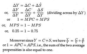
2. Columns (5), (7) and (8) show changes is the level of income, consumption and saving. Income change (∆Y) is the sum of the change in consumption (∆C) and the change in saving (∆S) i.e., ∆Y = ∆C 4- ∆S. (These three columns are set between the lines of the first three columns to indicate absolute changes in Y, C and S).

3. In this example, we assume that MPC is con­stant at all levels of income. It is 0.75. implying that one-fourth of every additional income is saved. When national income increases by Re. 1.00 consumption spending rises by 75 paise and saving by 25 paise. Since what is not spent on consumption goods is auto­matically saved the sum of the two marginal propen­sities is always equal to one. It is because

4. The fourth assumption that we have made earlier regarding the characteristics of consumption may now be verified from Table 32.2. By looking at Table 32.2 we discover the following:

(a) At the break-even level of income Y = C and S = 0. So APC = C/Y = 1 and APS = S/Y = 0. Thus, again APC + APS = 1.

(b) If actual income is less than the break-even level, saving is negative, or consumption is greater than income. Thus if C > Y. APC = C/Y is greater than one.

(c) If actual income is greater than the break-even level, exactly the opposite thing is observed. Since saving is positive, C is less than Y and APC = C/Y is less than one.

(d) Since the sum of MPC and MPS is always equal to one, MPC has to be less than one at all levels of income.

(e) Finally, we see that the MPS is constant at all levels of income (at 0.25) while the APS rises with income. In our example when Y — Rs. 1200 crores, APS is zero and when Y rises to Rs. 2000 crores, APS is positive (it increases from zero to 0.10).

Graphical Representation of Propensity to Consume and Save:

We may now illustrate the consumption propen­sities graphically. The graphs are drawn on the basis of data presented in Table 32.3. In Fig. 32.2 (i) we show a new consumption function. Point X on the function shows the case where income is Rs. 5 and consump­tion is Rs. 4. So the APC = 4/5 = 0.80.

Graphically APC is measured by the ratio of the length of the ver­tical line showing the amount of consumption at point x(C = 4), to the horizontal line showing the level of income at the point (y = 5). This ratio is given by the slope of the line drawn from the origin to the ref­erence point x. Many such lines can be drawn from the consumption function, shown in Fig. 32.2 (i) by choosing other reference points.

 

We may now look at point y. Now APC = 6/10 = 0.60 as Fig. 32.2 (i) shows. Here the APC is the slope of the line joining the origin to point y. In Fig. 32.2 (ii) we illustrate the MPC. Here ∆C is the vertical distance separating points X and y, while ∆y is the horizontal distance between the two points.

Thus, the slope of the line joining the two points x and y is ∆C/∆Y which is indeed the MPC, i.e., the ratio of the change in consumption to the change in income under consideration. Thus, the slope of the consumption function between two points being considered is the MPC.

If we assume linear consumption function, its slope will be the same at all points between x and y. But in reality we come across non-linear consumption functions due to declining MPC. If MPC falls with an increase in income MPC will be less than APC. In this case the MPC between two distinct points may be taken as the average slope of the consump­tion function between the points being considered.

Thus we may sum up the above two results shown graphically:

1. The APC at any point on the consumption function is measured by the slope of the line joining that point with the origin.

2. The MPC between any two points on the consumption function is measured by the slope of the line joining the two points.