Income and Consumption Function: Keynes Contribution | Consumption Function

Let us make an in-depth study of the Keynes Contribution towards the Concept of Income and Consumption Function.

The consumption function, the relationship between consumption and income, is largely a Keynesian contribution.

Before the 1930s, most economists stressed the relationship between consumption (or saving) and the interest rate. Keynes postulated that consumption depends mainly on income.

In regard to the relationship, he argued that consumption increases as income increases but by an amount less than the increase in income. Thus, Keynes assumed that the marginal propensity to consume is greater than zero and less than unity.

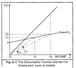
Keynes also argued that the average propensity to consume, the fraction of income consumed, decreases as income increases. For example, in Figure 6.11, the average propensity to consume or APC at income level Y₁ equals C₁ divided by Y_1. If C₁ equals Rs. 600 billion and Y₁ equals Rs. 800 billion, the APC is 0.75.

Mathematically, the APC equals C/Y. The APC also equals the tangent of the angle 9, where 0 is the angle between a line drawn from the origin to the combination of income and consumption in question and the horizontal axis. For example, at income level Y₁, the APC equals C₁/Y₁ or, alternatively, the tangent of angle θ₁. If income increases to Y₂, the APC equals C₂/Y₂ or, alternatively, the tangent of angle θ₂. Since angle θ₂ is less than angle θ₂, the APC at income level Y₂ must be less than the APC at income level Y₁.

The MPC and APC are often confused. The MPC equals ∆C/∆Y; the APC equals C/Y. Thus, the MPC is the slope of the consumption function, whereas the APC is the slope of the line drawn from the origin to the combination of income and consumption in question. In Figure 6.11, the MPC is constant and less than the APC.

Moreover, as income increases, the PC declines. In general, the MPC is not equal to the APC. Assuming the consumption function to be linear, the MPC equals the APC if and only if the consumption function passes through the origin.

The consumption function in Figure 6.11 reflects Keynes’s assumptions about the relationship between consumption and income. Specifically, the function is drawn so that the marginal propensity to consume is positive but less than 1 and the average propensity to consume decreases as income increases.

Early Keynesians were enthusiastic about Keynes’s contribution for two reasons. First, if a stable relationship between consumption and income exists, the amounts of investment, government purchases, and taxes necessary to provide for full employment may be determined. For example, sup­pose Y₂ represents the full employment level of income in Figure 6.11, and C = a + aY_d represents the consumption function for a given level of taxes.

The amounts of investment and government purchases necessary to achieve the full employment level of income Y₂ are represented by the distance between the 45° line and the consumption function. As a consequence, these amounts can be estimated. Policy makers can then take steps to achieve those levels.

Second, early Keynesians were enthusiastic because the initial empirical studies appeared to confirm the relationship. These early tests were based on cross-sectional budget studies. For groups of families, data were collected on size and disposition of income for a given period of time.

Almost without exception, these budget studies show a relationship between family consumption and family income like that which Keynes postulated for the economy. If a straight line is fitted to the data by regression analysis or some other statistical technique, the line intersects the vertical axis at a positive level of consumption and has a slope ranging from 0.6 to 0.8. Thus, the consumption-income relationship derived on the basis of budget studies appears to be consistent with the relationship postulated by Keynes.

Despite this evidence, it is not altogether clear that we can transfer estimates based on budget study data to the aggregate consumption function in which Keynes was interested. The cross-sectional data could show how family consumption varies as family income varies. Keynes’s hypothesis, however, relates to how aggregate consumption varies as aggregate income varies.

Since aggregate income is constant for the time span considered by budget studies, the budget studies shed little or no light on how aggregate consumption varies in response to variations in aggregate income. In fact, the aggregate relationship will show the budget studies relationship only under certain restrictive conditions. Even so, the same type of relationship appears in the aggregate data, provided that the study is confined to several decades or less.

Empirical Studies did Riot Support Keynes’s View:

After World War II, several occurrences cast some doubt on the usefulness and validity of the Keynesian consumption function First, economists using Keynesian consumption functions were unsuccessful in predicting postwar consumption. Their estimates were much less than the actual amounts. Second, in 1946, Simon Kuznets published time series data for the United States between 1869 and 1938 which showed the function to be linear ; however, the line was of the form C = b * Y_d.

In other words, a was approximately zero, contrary to the earlier assumption, which implies that the consumption function passes through the origin. Moreover, be was approximately 0.9 decidedly higher than reported earlier. This implies that the new function is steeper than the one originally assumed.

Thus, based on the empirical evidence, there appear to be two consumption functions:

(1) The short-run or cyclical consumption function based on budget study data and short-run aggregate data ;

(2) The long-run or secular consumption function based on Kuznet’s data.

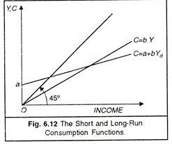
The short-run consumption function, shown in Figure 6.12 intersects the vertical axis at a positive amount of consumption a and is relatively fixed. The long- run consumption function, also shown in Figure 6.12, passes through the origin and is relatively steep.

In both cases, the marginal propensity to consume is constant. In the case of the short-run consumption function, the average propensity to consume decreases as income increases, whereas in the case of the long-run consumption function, the average propensity to consume is constant.

A number of hypotheses have been offered to explain consumer behavior and, at the same time, to reconcile the short-and long-run consumption functions. These contributions integrate the micro economics with macroeconomics. We now examine three of these hypotheses: the absolute, relative, and permanent income hypotheses given about the consumption function.