Consumption Function: Concept, Characteristics and Possibility

In this article we will discuss about the Consumption Function:- 1. Concept of Consumption Function 2. Characteristics of Consumption Function 3. Possibility.

Concept of Consumption Function:

J. M. Keynes first introduced the term ‘consump­tion function’ in 1936 to describe the relationship be­tween household’s planned consumption expendi­ture and all the above forces that determine it. In order to develop a theory we have to hold all the vari­ables, except one, constant. This will enable us to study how consumption varies with income.

On the basis of such study it will be possible for us to derive a simple relation between consumption and income. This relation was called by J. M. Keynes the consump­tion function and is expressed as: C = f(Y), where C is consumption and Y is income.

This relation implies that consumption depends on income or is a function of income. If there is a change in any other variable affecting consumption spending there will be a shift of the consumption function.

Induced Expenditure:

Since consumption depends on income and varies with income changes it is called induced expenditure. In Keynes’ theory of income determination variations in consumption are explained by changes in national income.

The Aggregate Consumption Function:

Every in­dividual or household has its own consumption func­tion. The function shows how its desired consump­tion expenditure varies with its income. By adding up the consumption functions of all households we arrive at the aggregate consumption function. This is of interest to us in macro-economics. It shows how the total desired consumption spending of all households varies with national income.

The aggregate consumption function reflects the behaviour of different types of individuals. However, extreme fluctuations cancel each other out. When, for example, income rises, some very poor people may spend all of the extra income, while some very rich ones may save all the extra income.

But since most people spend a portion of their extra income and save the rest, the aggregate consumption function shows the same type of behaviour, i.e., when national income rises there is an increase in both consumption and sav­ing.

From now onwards when we speak of the con­sumption function we shall be referring to be aggregate or macro function, i.e., consumption function for the whole economy.

Characteristics of Consumption Function:

A study of the short run consumption function reveals the following four characteristics:

1. Most poor people find it difficult to save be­cause they spend the major portion of their income on consumption goods. So income must reach a min­imum level for any saving to occur. In other words, there is a break-even level of income. It is the level of income at which households spend all of their income on consumption goods, neither more nor less, i.e., at which saving is zero.

2. Below the critical (break-even) level people plan to spend in excess of their current income.

This can be done in two ways:

(a) Either by borrowing or

(b) By dissaving, i.e., by spending out of wealth accu­mulated in the past.

However, there is a limit to the extent to which this process can go. People cannot consume indefinitely by borrowing or by reducing the stock of wealth. Since the stock of wealth is lim­ited it will get exhausted sooner or later. This is why this type of consumption behaviour is unlikely to be observed in the long run.

3. Once income crosses the break-even level, peo­ple plan to consume only a portion of their income and to save the remaining portion of it.

4. If income increases (decreases), consumption spending will also increase (decrease) though not pro­portionately. For example, if India’s national income increases by Rs. 1 crores per annum consumption spending of all households might increase by Rs. 80, 00,000 and saving by Rs. 20, 00,000.

These are Keynes’ four basic assumptions about the dependence of consumption and saving on in­come. These are illustrated in Table 32.1. Each row in the table shows desired consumption, and desired saving at each level of income.

The data of Table 32.1 may also be plotted graphically as in Fig. 32.1. The line plotted in Fig. 32.1 is a consumption function. Any point on the line shows planned consumption at each level of income.

The above four characteristics of the consump­tion function may now be illustrated with the help of both Table 32.1 and Fig. 32.1.

1. Firstly Fig. 32.1 shows that the graph of the consumption function is upward sloping, implying that as income increases consumption spending also increases. This makes it clear that consumption chan­ges are induced by income changes. However, total consumption has an autonomous (income-independent) component.

In Table 32.1 and Fig. 32.1 when national income is zero consumption spending is Rs. 300 crores. When income increases by Rs. 400 crores consumption increases by Rs. 300 crores. This part of total consumption at higher level of income is called autonomous (subsistence) consumption. This is the minimum amount people must consume, irrespective of income, in order to survive.

2. The second point to observe is that when na­tional income is Rs. 1200 crores, consumption expen­diture is also Rs. 1200 implying that saving is zero. This is the break-even level of income and is shown by point d in Fig. 32.1.

3. The third point to observe is that when national income is Rs. 800 crores consumption spending is Rs. 900 crores. Thus at this level of income there is dis­saving of Rs. 100 crores, implying that consumption expenditure exceeds income. This excess of consump­tion spending over income is financed by borrowing or reducing past saving. Point c in Fig. 32.1 illustrates the point.

4. The fourth point is that if income crosses a Crit­ical level (i.e., the break-even level) saving will be pos­itive. This is illustrated by point f in Fig. 32.1. Point f shows that when national income is Rs. 2000 crores, desired consumption spending is Rs. 1800 crores.

5. The final point to observe is that every time na­tional income increase by Rs. 400 crores consumption spending increases by Rs. 300 crores. Thus when in­come increases consumption spending also increase, though not proportionately.

Possibility Consumption Functions:

So long we have considered a linear consump­tion function as shown in Fig. 32.3.

(a) below. Keynes, however, pointed out that as income increases con­sumption expenditure also increases, though not pro­portionately. In other words, MPC falls. Fig. 32.3

(b) shows a non-linear consumption function which cor­roborates the declining MPC hypothesis.

However, for the sake of simplicity Keynes assumed linear con­sumption function in his theory of income and em­ployment.

Both types of consumption function shown in Fig. 32.3 are quite consistent with the four basic hy­pothesis. Both the functions have positive intercepts. The implication is that in each case APC exceeds unity at zero in­come. The positive slopes of both the curves imply that MPCs are positive at all levels of income.

In Fig. 32.3 (a) the consumption function C₀ is linear. The implication is the MPC is the same at all levels of income. However, APC continues to decline along the line C₀ as income rises. (The latter proposition may also be tested geometrically).

The non-linear consumption function C₁ exhibits declining APC and declining MPC as well. In fact, the slope of the consumption function measures MPC. In Fig. 32.3 (b) we observe that as income rises the slope of the line C₁ falls. In other words, the line C₁ becomes flatter. Thus, successive increases in income cause less and less increases in consumption spending.

We have noted that people spend a portion of their income and save the remaining portion of it. Thus, saving is a residue. Therefore, when people make decisions about consumption they automati­cally make decision about saving. In other words, people have to make only one decision: how to di­vide their incomes between consumption and saving.

In the language of Paul Samuelson, consumption and saving are mirror image concept. Table 32.1 illustrates these two concepts. The figures in Col. (3) are implied by the figures in the first two columns.

Just as consumption spending depends on in­come and the propensity to consume, saving behavi­our depends on income and the propensity to save. So like two consumption propensities there are two saving propensities as well. The average propensity to save (APS) is the ratio of total saving (S) to total income (Y), i.e., S/Y. It is the proportion of total income devoted to saving.

The marginal propensity to save (MPS) is the ratio of the (absolute) change in saving (∆S) to the (absolute) change in national income (∆Y) that brou­ght it about:

MPS = ∆S/∆Y

In Table 32.1 we have calculated the average and marginal propensities to save. We see that MPS (= 0.25) is constant at all levels of income but APS rises with income. For instance, when Y is Rs. 1200 crores APC is zero and when V rises to Rs. 2000 crores APS is positive at 0.10.

Problem 1:

For each of the following consumption functions, find the marginal propensity to consume, MPC = dC/dY.

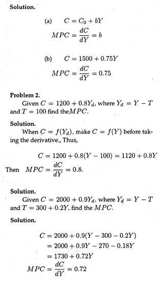
Problem 3:

Suppose planned consumption is given by the equation C = Rs. 40 + 0.75Y_d. Find planned con­sumption when disposable income is Rs. 300, Rs. 400 and Rs. 500.

Solution:

Substituting a Rs. 300 disposable income into the consumption equation, we have C = Rs. 40 + 0.75 (Rs. 300); C = Rs. 40 + Rs. 225 = Rs. 56. Consumption is Rs. 340 when Y is Rs. 400 and Rs. 415 when Y is Rs. 500.