In this article we will discuss about Consumer’s Equilibrium. After reading this article you will learn about: 1. Meaning of Consumer’s Equilibrium 2. Assumptions 3. Conditions 4. Corner Solutions.
Meaning of Consumer’s Equilibrium:
A consumer is in equilibrium when given his tastes, and price of the two fig 15 goods, he spends a given money income on the purchase of two goods in such a way as to get the maximum satisfaction, According to Koulsayiannis, “The consumer is in equilibrium when he maximises his utility, given his income and the market prices.”
Assumptions of Consumer’s Equilibrium:
The indifference curve analysis of consumer’s equilibrium is based on the following assumptions:
(1) The consumer’s indifference map for the two goods X and Y is based on his scale of preferences for them which does not change at all in this analysis.
ADVERTISEMENTS:
(2) His money income is given and constant. It is Rs.10 which he spends on the two goods in question.
(3) Prices of the two goods X and Y are also given and constant. X is priced at Rs.2 per unit and Y at Re. 1 per unit.
(4) The goods X and Y are homogeneous and divisible.
(5) There is no change in the tastes and habits of the consumer throughout the analysis.
ADVERTISEMENTS:
(6) There is perfect competition in the market from where he makes his purchases of the two goods.
(7) The consumer is rational and thus maximises his satisfaction from the purchase of the two goods.
Conditions of Consumer’s Equilibrium:
There are three conditions for consumer’s equilibrium:
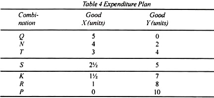
(1) The Budget line should be Tangent to the Indifference Curve. Given these assumptions, the consumer can buy 5 units of X by spending the entire sum of Rs. 10 on good X or on 10 units of Y. Table 15.4 illustrates some of the possible combinations on which Rs. 10 can be allocated.
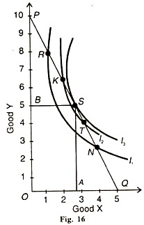
Fig. 16 shows these seven possible combinations indicated by points P, R, K, S, T, N and Q. The line PQ shows combinations of goods X and Y, given their prices, when he spends his income on them. This is because, algebraically I = Px. X + P .Y, where I represents the consumer’s income P and P the prices of goods X and Y, respectively.
This budget equation is the equation of the line connecting the points Q and P, where Q = I/Px and P = I/Py Thus PQ is the budget line.
On this budget line, the consumer can have any combination, out of the possible seven combinations P, R, K, S, T, N, or Q. Combination P or Q is out of question for in either case he would have only Y or only X. He would not take combination R or N on a lower indifferences curve f because combination K or T is also available to him on a higher indifference curve I2 .
But there is another combination S which is on the highest indifference curve I3, on this budget line PQ.
Since all other combinations lie on lower indifference curves, they represent lower levels of satisfaction than combination S which is the consumer’s equilibrium point. We may thus enumerate the conditions of consumer’s equilibrium.
The consumer is in equilibrium when his budget line is tangent to an indifference curve. PQ is tangent to curve I, at S. At point S, he is also satisfying the budget equation
I (Rs 10) = OA. P + OB.PY
= 2½ units of X. Rs. 2 + 5 units of Y. Re 1
ADVERTISEMENTS:
= Rs 5 + Rs 5
= Rs 10
(2) At the point of Equilibrium the Slope of the Indifference Curve and of the Budget Line should be the same. At S, the slope of the indifference curve is, in fact, the marginal rate of substitution of X for Y and on the budget line it is the ratio of the price of X to the price of Y. The slope of the budget line
PQ = I/Р / I/P = I/PY x YPX/I= PX/PY
ADVERTISEMENTS:
And the slope of I’ curve is MRSXY .
Thus MRS x =PX/P at point S in Fig. 16.
This is a necessary but not a sufficient condition for consumer’s equilibrium.
(3) Indifference curve should be Convex to the Origin. Therefore, the last conditions are that at the point of equilibrium, the marginal rate of substitution of X for Y must be falling for equilibrium to be stable. It means that the indifference curve must be convex to the origin at the equilibrium point.
ADVERTISEMENTS:
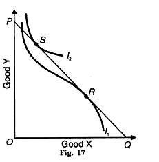
If the indifference curve is concave to the origin at the point R, the MRSXY increases. The consumer is at the minimum point of satisfaction at R on the concave I1 curve in Fig. 17.
A movement away from R toward either axis along PQ would lead him to higher indifference curve. Point S on the curve I2 is, in fact, the point of maximum satisfaction and of stable equilibrium.
Thus for equilibrium to be stable at any point on an indifference curve, the marginal rate of substitution between any two goods must be diminishing and be equal to their price ratio i.e. MRS’ = Px/Py Therefore, the indifference curve must be convex to the origin at the point of tangency with the budget line.
Corner Solutions of Consumer’s Equilibrium:
We have seen above that the point of tangency between the budget line and a convex indifference curve leads to consumer’s equilibrium when he buys some units of both the commodities. This is called the interior solution, as at point 5 in Figure 17 which lies in the interior of the commodity space.
We also observed that if the indifference cure is concave to the origin, the consumer cannot be in equilibrium at the point of tangency with the budget line, as at point R in Figure 17 because the MRSxy increases as we move to the right or left of this point.
ADVERTISEMENTS:
However, it can be shown in terms of straight line, concave and convex indifference curves that the consumer can be in equilibrium when he consumes only one good instead of two goods available to him. In all these cases, the consumer’s equilibrium will be a corner solution. But the condition that MRS must equal Px/Py at the point of equilibrium is not fulfilled. We discuss these cases below.
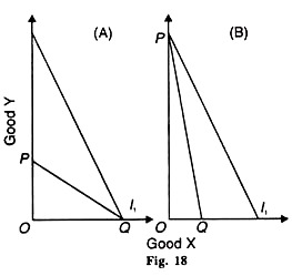
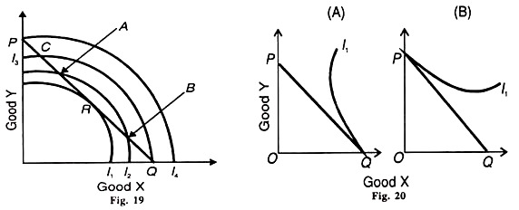
1. In the case of a straight line indifference curve, if the budget line is relatively less steep than the indifference curve, the equilibrium will be in the corner where the I1, curve meets point О of the budget line PQ and the consumer will buy OQ and the consumer will buy OQ of good X and none of Y, as shown in Figure 18 (A).
On the other hand, if the budget line PQ is steeper than the curve I1, as shown in panel (B), the equilibrium will be at the P corner and the consumer buys OP of good Y and none of X.
2. To analyse the case of a concave indifference curve, consider Figure 19 where the curve I1, is tangent to the budget in PQ at point R. But R is not the point of maximum satisfaction for the consumer because by moving outwards along the budget line away from R and towards one of the axis, the consumer’s satisfaction can be increased.
Points A and В are available to him because they are on the higher indifference curve I2. But he can increase his satisfaction further by moving to point С on the more higher curve I3, and further to point P on the highest indifferences curve I4,.
ADVERTISEMENTS:
The consumer will thus be in equilibrium at the corner point P of the indifference curve and the budget line PQ and consume only OP quantity of good Y and none of good X. If the consumer wishes to consume only good X, the corner solution will be at point Q on the indifference curve I3.
3. There may be a corner solution even when an indifference cure is convex to the origin. This happens in the case of many goods when their prices are so high that the consumer can buy only one good at a time with his given money income.
Such goods may be a car, a colour TV, or a VCR, etc. Consider Figure 20 (A) where the slope of the budget line PQ is less steep than the curve I1 (or the curve is steeper than the line PQ). The equilibrium will be at the corner point Q where the consumer spends his entire income in buying OQ of X and none of Y.
On the other hand, in panel (B) of the figure, the budget line PQ is steeper than the curve I1;(or the curve I1 is flatter than the line PQ) and the consumer’s equilibrium will be at the corner point P where he spends his entire income in buying only OP of Y and none of X. Each of the corner solutions Q and P is the closet to the tangency equality of the budget line and the indifference curve that the consumer can achieve.
Thus convex indifference curves are capable of explaining interior as well as corner solutions.
