The Budget Equation and the Budget Line by Consumers

In this article we will discuss about the budget equation and the budget line by consumers.

The preference-indifference pattern of the consumer based on the axioms of preferences. The indifference map of the consumer shows that the points lying on any particular IC give the consumer the same level of utility. It also shows that the points lying on a higher IC give the consumer a higher level of utility than the points on a lower IC.

Therefore, the points on the former curve are strictly preferred to the points on the latter curve. The consumer would always want to climb up on a higher IC because then he would be able to obtain a higher level of utility. But the real world consumer is constrained by his income or budget.

His income may not permit him to climb on the ICs beyond a certain height. The consumer’s income and the prices of the goods together give us the budget constraint of the consumer, and his budget is as important as his preference-indifference pattern in the determination of his behaviour in the market. 

The Assumptions of Budget Equation and the Budget Line:

While discussing the budget of the consumer, for the present, assume the following:

(i) The prices of the two goods (X and Y) have been determined in the market, and they are given and constant for the consumer.

(ii) The consumer has a fixed amount of money income to spend on the two goods.

(iii) Both the goods are MIBs.

(iv) The consumer wants to maximise utility.

(v) He spends all his money on the goods because of (iii) and (iv).

(vi) He can purchase any combination of the goods if his budget permits, i.e., there are no (absolutely) maximum limits on the purchase of the goods.

The above assumptions would lead to the properties of the budget equation and the budget line of the consumer.

The Properties of the Budget Equation and the Budget Line:

Suppose that the consumer’s money income is denoted by M and the prices of the goods are given to be p_x and p_y.

Then the equation M = p_x. x + p_y . y ……(6.14)

is known as his budget equation.

As is evident from (6.14), the budget equation is linear in

M̅, x and y, p_x and p_y being given and constant. Now, assume that the consumer’s money income is fixed at M, then from his budget equation (6.14), is known as his budget line.

The equation of the budget line would be:

M̅ = p_x.x + p_y.y …..(6.15)

Since M̅, p_x and p_y are constants, (6.15) is a linear equation in x and y, i.e., it is the equation of a straight line in a two dimensional commodity space. The budget line gives us the combinations of x and y that the consumer can purchase with his fixed money income M.

It may be noted that equation (6.14) represents a family of parallel budget lines. Because, at each value of M, a separate budget line from this equation and the slope of each such budget line, is −p_x/p_y = constant (p_x and p_y remain constant).

The equation of the budget line is:

M̅ = p_x.x + p_y.y [eq. (6.15)]

The features of this line are:

(i) It is a straight line in the commodity space, since it is a linear equation in x and y.

(ii) Its slope is negative being equal to − p_x/p_y (^._.^. p_x, p_y > 0).

Therefore, the numerical slope of the budget line is p_x / p_y which is equal to the ratio of the prices of X and Y. Since the numerical slope of the line represents the price ratio, or, the relative price of good X in terms of good Y, this line is also called the price line.

(iii) The intercept form of the budget line is:

This gives the x-intercept of the budget line is M̅ / p_x which is equal to the quantity of good X that the consumer would be able to buy if he spends all his money income (M) on X. Similarly, the y-intercept of the budget line is M / p_y which is equal to the quantity of good Y that the consumer would be able to buy with all his money income.

(iv) Since M̅, p_x and p_y are given, can immediately know the intercepts M̅/p_x and M̅/ p_y, and is also know the meeting points of the budget line with the x-axis and y- axis. These points would be (M̅/p_x, 0) and (0, M̅/p_y) respectively.

By joining these two points at once have the budget line of the consumer. It may be noted here that, at the point (M̅/p_x, 0), the consumer would buy only good X, and the point (0, M̅/p_y), he would by only good Y. At all other points on the line he would buy a combination of the goods.

The concept of the budget line can be illustrated with the help of a simple example. Suppose M̅ = Rs 500, p_x =  Rs 10 and p_y = Rs 5. Then, putting these values in (6.15), the budget line of the consumer as 500 = 10x + 5y (6.17)

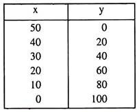
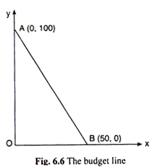
The x-intercept of the budget line (6.17) = M̅/p_x = 500/10 = 50 is obtained, i.e., the consumer would be able to buy 50 units of good X with all his income; and the y-intercept of the line = M̅/p_y = 500/5 = 100, i.e., the consumer would be able to buy 100 units of good Y with all his income. Therefore, (50, 0) and (0, 100) are the two combinations that lie on the line which has been shown in Fig. 6.6. Some other combinations along with these two have been shown in the Table 6.1.

Table 6.1 Some of the Combinations of Goods that Lie on the Budget Line in Fig. 6.6

(v) Lastly, the slope of the budget line is –p_x/p_y = -10/5 = -2 and the numerical slope of the line is –p_x/p_y = 2/1 = 2:1 which is the ratio of the prices of the goods X and Y. This price ratio represents the relative price of good X in terms of (the quantities of) good Y. Here, in the market, price of one unit of good X is 2 units of good Y.