
In a model of collusive oligopoly, we discuss the economics of agreement between the firms in an undifferentiated oligopolistic industry. When these firms get together and agree to set prices and outputs so as to maximise total industry profits, they are known as a cartel.
Assumptions of the Cartel Model:
For the sake of simplicity, we shall make here the following assumptions:
(i) There are only two firms in the oligopolistic industry, i.e., here we have a case of duopoly.
(ii) Each firm produces and sells a product that is a perfect substitute for that of the other.
ADVERTISEMENTS:
(iii) The product is perishable.
(iv) There are many knowledgeable buyers of the product.
(v) Each firm knows the market demand for the product.
(vi) The two firms have different cost curves.
ADVERTISEMENTS:
(vii) Both the firms have the same expectations about the prices and productivities of the inputs which they use.
(viii) The price of the product is the sole parameter of action of each firm.
(ix) The two firms are contemplating whether or not to form a cartel and agree upon a price that will promise the maximum maximorum of profits per period to both of them jointly.
Analysis of the Cartel Model:
Let us discuss the choice of this price [mentioned in assumption (ix)] and its implications with the help of Fig. 14.16. Here, in part (a), the average and marginal cost curves of duopolist A are given to be ACA and MCA, and those of duopolist B are given to be ACB and MCB in part (b).
ADVERTISEMENTS:
As is seen in these figures in 14.6, the cost levels of A have been assumed here to be lower than those of B. The curve DD in part (c) of the figure is the market demand curve for the product produced by the duopolists.
Here the dupolists A and B are exploring the possibility of jointly producing and selling the product and earning the maximum maximorum of profits. Henceforth, we shall call the duopoly firms A and B that have come under collusion, the firms A + B (the “plus” sign indicates collusion).
In our attempt to analyse the price-output-profit policy of the firms A + B, we shall first see how the firms would distribute the production of any particular quantity (q) of their product between the plants of A and B, so that the cost may be minimum. We may call the plants of the two firms plant A and plant B.
Now, the total cost (C) of producing any particular quantity of output, q is
c = CA(qA) + CB(qB) = C(qA, qB) (14.72)
subject to
q = qA + QB = constant (14.73)
where qA = quantity of output to be produced in plant A,
and qB = quantity of output to be produced in plant B,
ADVERTISEMENTS:
CA = cost of production in plant A
and CB = cost of production in plant B
Given these, the first-order conditions (FOCs) of producing the output quantity, q, in the two plants at minimum cost, i.e., the FOCs for minimising C, are
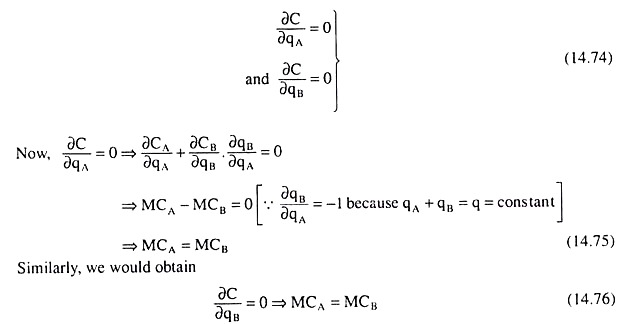
ADVERTISEMENTS:
Conditions (14.75) and (14.76) give us that two (or more) oligopoly firms under collusion (here firms A + B) would distribute the production of any particular quantity of output between their plants in such a way that the marginal cost (MC) in each plant may become the same.
We may easily understand the economic significance of this condition. Instead of MCA being equal to MCB, if we have MCA > MCB (in the two-firm case), then the firms A + B would reduce the quantity of production in the higher cost plant A and increase the quantity in the lower cost plant B, total output remaining the same.
The firms would do this because then they would be able to produce the same quantity of total output (q) at a lower cost.
Now, as we know, for the sake of profit maximisation, and, therefore, for the sake of efficient production, firms A + B would operate along the upward sloping segments of the MC curves of plants A and B that correspond to the second stage of production. That is why, as the firms decrease and increase qB, MCa will fall and MCB will rise, and ultimately, at some distribution, MCA will become equal to MCB.
ADVERTISEMENTS:
This distribution is the cost-minimising distribution of the output quantity, q, between the two plants. For if MCA = MCB, then it will not be possible for the firms to reduce the cost further by transferring output production from plant A to plant B, or, the other way round.
On the other hand, if MCA < MCB, the firms A + B will reduce output in plant B and increase it in plant A, till MCA rises and MCB falls to become equal to each other.
Thus, we come to the conclusion that the duopoly firms under collusion (i.e., firms A + B) will distribute the production of any particular quantity of output over the two plants in such a way that the MC in each plant may become the same; only then it would be able to produce the said quantity at the minimum cost.
Therefore, that at each quantity of output, q, there is a problem of cost- minimisation, or, profit-maximisation (the price, p, and, therefore, total revenue, p x q, being given by the demand curve). Here equilibrium will be obtained at that quantity, q*, at which profit is maximum among the maximums, or, maximum.
We may now proceed to explain how the equilibrium output, q*, of the firms A + B with maximum of profit is obtained. It follows from (14.75) or (14.76) that, at any output, q = qA + qB, the condition MCA = MCB ensures cost-minimising of profit-maximising distribution of q between the two plants.
Now, at any q = qA + qB, the MC of firms A + B is MCA = MCB. This is because, here the qAth unit of output is either the qAth unit of output in plant A or the qBth unit of output in plant B, and the additional cost of producing that unit is either MCA or MCB, and MCA = MCB.
ADVERTISEMENTS:
On the revenue side, the firms A + B sell any quantity, q, of their product at the price given by the demand curve, DD. Now, if at any q, the firms A + B have MC = MCA = MCB < MR (marginal revenue), then they would be able to earn a positive profit on the margin, and so, they would increase the output to push up the maximum maximorum of profit.
But as q increases the MR, being a decreasing function of q, would diminish, and MC (= MCA = MCB) would increase, since in the relevant range, both MCA and MCB are increasing functions of q. Therefore q, while increasing, would eventually assume a value (say, q*) at which we would have MR = MC (= MCA = MCB).
At this q = q*, the firm would acquire the maximum maximorum of profit. For, now its profit on the margin is zero, and so it will not be able to increase its profit by increasing q.
On the other hand, if at some q, the firms have MC = MCA = MCB > MR, then it would suffer losses on the margin and would now want to shed the loss-earning marginal units, i.e., it would now want to decrease q to maximise its profit. But as q decreases, the firm’s MC (= MCA = MCB) would also decrease, and its MR would increase.
Eventually, at q = q*, the firm would have MR = MC (= MCA = MCB), and this q = q* would be its q with maximum of profit. For, now the firms’ losses on the margin are zero, and so it is no longer required of the firms to decrease their output in order to maximise profit.
It follows from the above analysis that the necessary or the first order condition (FOC) for profit maximisation under collusive oligopoly (here duopoly) is
ADVERTISEMENTS:
MR = MCA = MCB (14.77)
However, condition (14.77) is not the sufficient condition or the second order condition (SOC) of profit maximisation. For, if at the MR = MCA = MCB point, the firms A + B find that a further increase in output would result in MC (= MCA = MCB) being less than MR, (which can of course happen in an inefficient stage of production), then the firms would not settle at this point, rather they would go on increasing the output quantity, for, by doing that, they would be able to increase the profit level.
Therefore, the SOC for profit maximisation states that at the point where the FOC is satisfied, i.e., at the MR = MCA = MCB point, further increase in output should result in MC = MCA = MCB being greater than MR. In that case, there would be a loss on the margin and so the firms A + B would not venture beyond the point (where the FOC is satisfied).
In other words, the SOC for profit maximisation under collusive oligopoly states that, at the point of intersection between the MC curve and the MR curve, where the FOC has been satisfied, the slope of the MC curve viz., the MCA + B curve in Fig. 14.16(c), which, as we shall see, is the lateral summation of the MCA and MCB curves, should be greater than that of the MR curve.
It may be noted that, since the firms operate in the stage of efficient production, they would operate along the positively sloped portion of their respective MC curves, and, therefore, along the positively sloped portion of the MCA + B curve. Here the SOC for profit maximisation would be automatically satisfied, for the MR curve of the firms A + B is negatively sloped, by definition.
We may now illustrate the profit-maximising equilibrium of the collusive oligopoly under discussion with the help of Fig. 14.16. The MCA+B curve in Fig. 14.16(c) is the MC curve of firms A + B. It is obtained by laterally adding together the MCA and MCB curves given in Figs. 14.16(a) and 14.16(b). The curve MCA+B shows us what would be the total output of the firms A + B at any particular amount of MC in both the plants.
ADVERTISEMENTS:
Thus, if the MC in both the plants is to be OC, (MCA = MCB = OC), plant A should produce OMA of output and plant B should produce OMB. The combined output in this case would be OMA + OMB = OM (in Fig. 14.16).
Conversely, we would also know from the curve MCA+B what would be the MC = MCA = MCB at any particular output. For example, at q = OM, the MC = MCA = MCB would be OC, provided the distribution of this q between the two plants is qA = OMA and qB = OMB.

Now, the total output for which the firms A+ B would be jointly earning the maximum maximorum of profits is obtained at the point of intersection, E, of the MR and MCA + B curves in Fig. 14.16 (c). For at the point E, or at the total output of OM, the FOC for profit maximisation, viz., MR = MCA = MCb (- OC), has been satisfied.
Also, the SOC for maximum profit has been satisfied at point E, for here the MR curve is negatively sloped and the MCA + B curve is positively sloped.
It is obtained from the AR curve in Fig. 14.16(c) that the output OM of firms A + B can be sold at the price OR The output OM and the price OP are called, respectively, the monopoly output and price, for they would form the equilibrium price-output combination if the firms A and B merged into a single monopolistic firm.
ADVERTISEMENTS:
The duopolists in this collusive oligopoly model will plan to sell OM units of their product at a price of OP per unit and firm A will produce and sell OMA units per period and firm B, OMB per period. The distribution of the ‘monopoly’ output of OM between the two firms implies a distribution of the maximum joint profits.
In the solution given in Fig. 14.16, firm A may expect to earn LMNP of profits per period and firm B may expect to earn RSTP of profit per period. The sum of LMNP and RSTP will be the maximum maximorum of profits that the two firms will be able to earn jointly.
Mathematical Derivation of the Condition for Maximum Profit:
We may also derive the conditions for maximum maximorum of profit under collusive oligopoly with the help of calculus.
The profit (π) function of the firms A + B is:
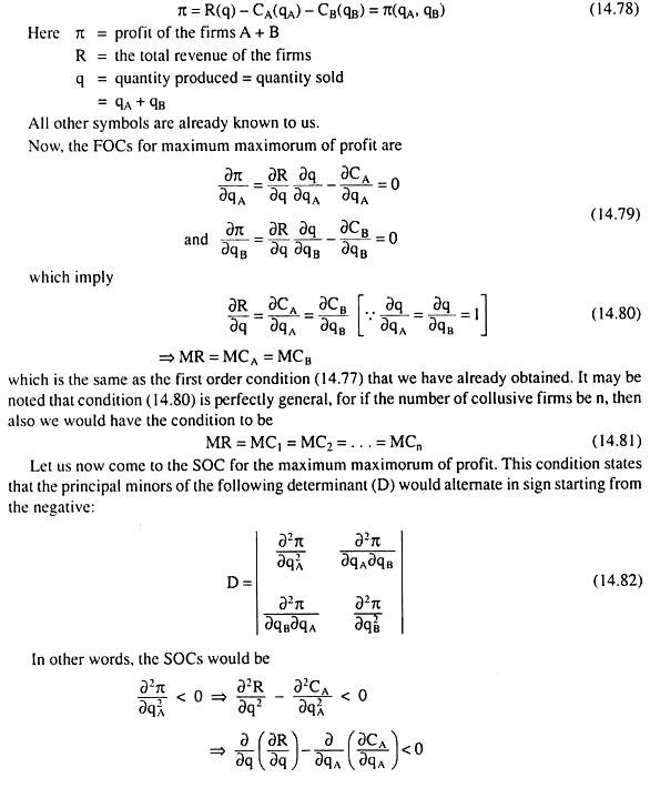
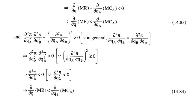
(14.83) and (14.84) give us the SOCs for maximum maximorum of profit under collusive oligopoly. These conditions state that at the MR = MCA = MCB point, i.e., at the point of intersection of the MR and MCA + B curves in Fig. 14.16 (where the FOC has been satisfied), the slope of the MR curve of firms A + B should be less than the slopes of both MCA and MCB curves.
This implies, as we have already asserted, that the slope of the MR curve should be less than the slope of the MCA+B curve. We have also mentioned the significance of these conditions. Like the FOC, the SOCs are also perfectly general.
That is, if the number of collusive firms is n, then these conditions give us that, at the point where the FOC is satisfied, the slope of the MR curve should be less than the slope of the MC curve of each of then firms.
Comparison between the Collusion Solution and the Quasi-competitive solution:
We may now obtain the collusion solution for the example given in (14.5) and compare it with the quasi-competitive solution given in (14.8).
The profit of the two firms taken together, or, the industry profit, is given by
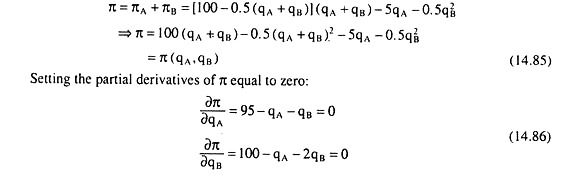
Solving (14.86) for qA and qB and substituting in equations (14.5), (14.85) and (14.86), we have the following collusive solution:
qA = 90 (units), qB = 5 (units), p = 52.5 (Rs), πA = 4,275 (Rs), πB = 250 (Rs.). (14.87)
Comparing (14.87) with (14.8), we find that, under collusion, total output is much lower (95 < 190), price is much higher (52.5 > 5) and profits are much higher (4,275, 250 > 0, 12.5).
Cartel Instability:
The problem with agreeing to form a cartel in the real world is that there is always a temptation for the participating firms to act contrary to the agreement, i.e., to cheat. We may elaborate the problem as follows. Let us rewrite the profit function (14.78) as
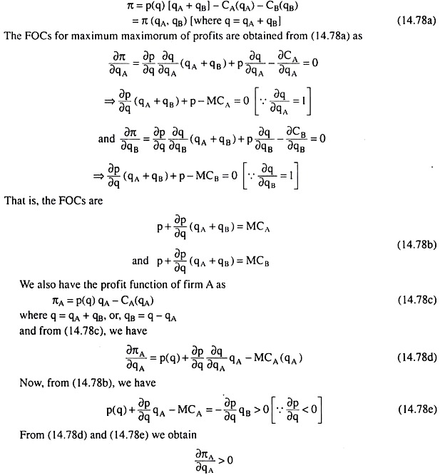
That is, if firm A believes that firm B will keep its output fixed, then it will also believe that it can increase profits (πA) by increasing its own production (qA). It may be shown in a similar way that the firm B will also believe accordingly.
And herein lies the temptation for a member of the cartel to increase his own profits by unilaterally expanding his output beyond the output level that maximises joint profits. The situation becomes grave for the existence of the cartel if each firm comes to know that the other firm is not going to keep its output at the agreed level.
Therefore, in order to make the cartel effective and operational, its members must be able to detect and punish cheating. Otherwise, temptation to cheat would break the cartel.
In order to renew our understanding of the cartel solution, let us assume that the costs of production are zero and the demand curve for the product is linear which is the same as (14.9).
Then the total revenue (R) function of the cartel will be
R = (a – bq)q = aq – bq2 = R(q) where q = qA + qB
And here the MR = MC condition, or the FOC for maximum profit, will be
a – 2bq = 0
⇒ a – 2b(qA +qB) = 0
⇒ qA + qB = a/2b
Since marginal costs are zero here, the division of output between the two firms does not matter. All that is important here is the total industry output which is This solution is shown in Fig. 14.17. In this figure, qA is measured along the horizontal axis and qB along the vertical axis.
Since qA + qB = a/2b, here we have qA = a/2b, given qB = 0 and qB = a/2b, given qA = 0, or here we would have any other combination of positive values of both qA and qB provided it lies on the straight line joining the points L (a/2b, 0) on the horizontal axis and M (0, a/2b) on the vertical axis.
Now, at any point on this line, the industry’s profit is maximum, i.e., the profit of A is maximum given the profit of B and the profit of B is maximum given the profit of A, i.e., the iso-profit curve of A is the lowest, given the iso-profit curve of B and the iso-profit curve of B is the lowest, given the iso-profit curve of A, i.e., at any point on the line LM, the iso-profit curves of the two firms are tangent to each other.
Hence, the (qA, qB) combinations that maximise total industry profits and give us the alternative cartel solutions are those that lie on the line LM in Fig. 14.17.
Fig. 14.17 also helps us to understand how the temptation to cheat is present at the cartel solution. Let us consider, for example, the point N at the midpoint of the line segment LM.
At this point, the two firms share the market equally between themselves, each producing and selling half of the total quantity sold in the market. Let us now suppose that firm A decides to increase its output believing that B would keep its output unchanged.
Consequently, A would now move towards right of the point N along a horizontal straight line and would reach a lower iso-profit curve which implies that he would now be on a higher level of profit.
Similarly, if firm B decides to increase its output at the point N, believing that A would keep its output constant, it would move upward from N along a vertical straight line and reach a lower iso-profit curve or a higher level of profit. Thus both the duopolists are in temptation to increase their respective outputs in violation of the cartel agreement.

Punishment Strategies:
We have seen above that a cartel is fundamentally unstable for its members are always tempted to increase their output quantities beyond their maximising levels. If the cartel is to continue its operations successfully, the behaviour of its members must conform to the agreement made by them. One way to ensure this is for the firms to threaten to punish each other for violating the cartel agreement.
This is known as a punishment strategy. For example, let us consider a duopoly with two identical firms. If the firms come to an understanding and produce the monopoly output, then the share of each firm will be half the monopoly output (= 1/2 x 1/2 a/b = 1/4 a/b) and the total profit of the duopolists will be maximised.
Let us suppose that the profit accruing to each firm, now, is πm. In an effort to make this position stable, one of the firms, say, firm A, may threaten firm B that if it violated the output agreement, then it would punish firm B by producing the Cournot level of output forever.
Now, since the optimal response to Cournot behaviour is Cournot behaviour, both the firms now would operate at the Cournot equilibrium point which is the point of intersection, I, of the reaction functions of the two firms (not shown in Fig. 14.17). In other words, the point of operation of the firms would shift from the point N to the point I.
Consequently, both the firms would move to a higher iso-profit curve, i.e., both of them would move to a lower level of profit. It may be noted also that in the cartel solution, total amount of output produced by the duopolists was 1/2 of competitive output and each of them had an equal share which was 1/4 of the competitive output.
Now, in the Cournot solution, total amount of output is larger being equal to 2/3 of competitive output and each firm had an equal share, equal to 1/3 of competitive output. Therefore, as the cartel breaks down, the firms now produce a larger quantity of output and sell at a lower price, since the demand curve for the product is negatively sloped, and earn a lower level of profit.
The economics here is very simple. Let us suppose that the two firms have agreed to produce an equal share of the collusive, monopoly level of output. Now, if one of the firms produces more output than its quota, it makes profit, say, πd where πd > πm.
That is, here the two firms agree to enter into a cartel. They agree to restrict production. Consequently, the price goes up. Now one of them decides to produce more output to take advantage of the high price. This is the standard temptation that a cartel member is easily susceptible to.
Let us now look at the benefits and costs of cheating as opposed to those of normal cartel behaviour. If each firm produces the cartel amount, then it gets a steady stream of payoffs of Tin,. The present value (PV) of this stream is given by PV of Cartel behaviour = πm + πm/r.
On the other hand, if the firm produces more than the cartel amount, it gets a one-time benefit of profits πd, but then the cartel breaks up, and it would have to revert to the Cournot behaviour to get a stream of payoffs of πc. Therefore, we have
PV of cheating = πd + πc/r
Obviously, the PV of cartel amount would be greater than the PV of cheating if
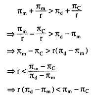
The above inequality implies that so long as the interest rate (r) is sufficiently small, the expected return from cheating (i.e., the LHS of the inequality) is smaller than the expected return of cartel over the Cournot return (i.e., the RHS of the inequality), and therefore, if the above inequality is satisfied, the tendency to violate the provisions of the cartel agreement would be eliminated. That is, the firms would now stick to their cartel quotas.