As price of a good X falls, other things remaining the same, consumer would move to a new equilibrium position at a higher indifference curve and would buy more of good X at the lower price unless it is a Giffen good.
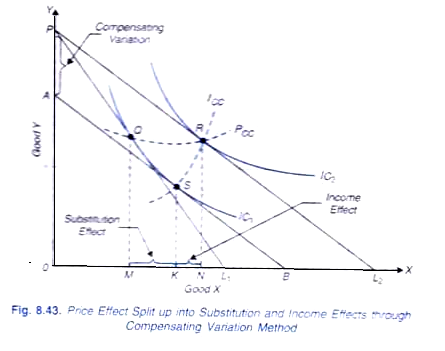
Thus, in the Fig. 8.43 the consumer who is initially in equilibrium at Q on indifference curve IC1 moves to the point R on indifference curve IC2 when the price of good X falls and the budget line twists from PL1 to PL2.
The movement from Q to R represents the price effect. It is now highly important to understand that this price effect is the net result of two distinct forces, namely substitution effect and income effect. In other words, price effect can be split up into two different parts, one being the substitution effect and the other income effect.
There are two approaches for decomposing price effect into its two parts, substitution effect and income effect. They are the Hicksian approach and Slutsky approach.
ADVERTISEMENTS:
Further, Hicksian approach uses two methods of splitting the price effect, namely:
(i) Compensating variation in income
(ii) Equivalent variation in income.
Slutsky uses cost-difference method to decompose price effect into its two component parts. How the price effect can be decomposed into income effect and substitution effect by the Hicksian methods is explained below.
1. Breaking up Price Effect: Compensating Variation in Income:
ADVERTISEMENTS:
In the method of breaking up price effect by compensating variation we adjust the income of the consumer so as to offset the change in satisfaction resulting from the change in price o a good and bring the consumer back to his original indifference curve, that is, his initial level of satisfaction which he was obtaining before the change in price occurred. For instance, when the price of a commodity falls and consumer moves to a new equilibrium position at a higher indifference curve his satisfaction increases.
To offset this gain in satisfaction resulting from a fall in price of the good we must take away from the consumer enough income to force him to come back to his original indifference curve. This required reduction in income (say, through levying a lump sum tax) to cancel out the gain in satisfaction or welfare occurred by reduction in price of a good is called compensating variation in income.
This is so called because It compensates (in a negative way) for the gain in satisfaction resulting from a price reduction of the commodity. How the price effect is broken up into substitution effect and income effect through the method of compensating variation in income is illustrated in Fig 8.43.

Now, if his money income is reduced by the compensating variation in income so that he is forced to come back to the original indifference curve IC1 he would buy more of X since X has now become relatively cheaper than before. In Fig. 8.43 as result of the fall in price of X, price line switches to PL2. Now, with the reduction in income by compensating variation, budget line shifts to AB which has been drawn parallel to PL2 so that it just touches the indifference curve IC1 where he was before the fall in price of X.
ADVERTISEMENTS:
Since the price line AB has got the same slope as Pig, it represents the changed relative prices with X being relatively cheaper than before. Now, X being relatively cheaper than before, the consumer in order to maximise his satisfaction in the new price income situation substitutes X for Y.
Thus, when the consumer’s money income is reduced by the compensating variation in income (which is equal to PA in terms of Y or L2B in terms of X), the consumer moves along the same indifference curve IC1 and substitutes X for Y. With price line AB, he is in equilibrium at S on indifference curve IC1 and is buying MK more of X in place of Y. This movement from Q to S on the same indifference curve IC1 represents the substitution effect since it occurs due to the change in relative prices alone, real income remaining constant.
If the amount of money income which was taken away from him is now given back to him, he would move from S on indifference curve IC1 to R on a higher indifference curve IC2. The movement from Son a lower in difference curve to R on a higher in difference curve is the result of income effect. Thus the movement from Q to R due to price effect can be regarded as having been taken place into two steps first from Q to S as a result of substitution effect and second from S to R as a result of income effect. In is thus manifest that price effect is the combined result of a substitution effect and an income effect.
In Fig. 8.43 the various effects on the purchases of good X are:
Price effect = MN
Substitution effect = MK
Income effect = K/V
MN = MK+KN or
ADVERTISEMENTS:
Price effect = Substitution effect + Income effect
From the above analysis, it is thus clear that price effect is the sum of income and substitution effects.
2. Breaking up Price Effect: Equivalent Variation in Income:
As mentioned above, price effect can be split up into substitution and income effects” through an alternative method of equivalent variation in income. The reduction in price of a commodity increases consumer’s satisfaction as it enables him to reach a higher indifference curve. Now, the same increase in satisfaction can be achieved through bringing about an increase in his income, prices remaining constant.
The increase in income of the consumer prices of goods remaining the same, so as to enable him to move to a higher subsequent indifference curve at which he in fact reaches with reduction in price of a good is called equivalent variation in income because it represents the variation in income that is equivalent in terms of gain in satisfaction to a reduction in price of the good.
ADVERTISEMENTS:
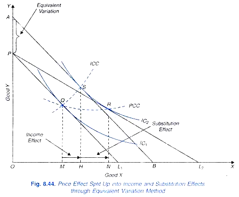
Thus, in this equivalent income-variation method substitution effect is shown along the subsequent indifference curve rather than the original one. How this price effect is decomposed into income and substitution effects through equivalent variation in income is shown in Fig. 8.44.
When price of good X falls, the consumer can purchase more of both the goods, that is, the purchasing power of his given money income rises. It means that after the fall in price of X if the consumer buys the same quantities of goods as before, then some amount of money will be left over. In other words, the fall in price of good X will release some amount of money. Money thus released can be spent on purchasing more of both the goods.
It therefore follows that a change in price of the good produces an income effect. When the power to purchase goods rises due to the income effect of the price change, the consumer has to decide how this increase in his purchasing power is to be spread over the two goods he is buying. How he will spread the released purchasing power over the two goods depends upon the nature of his income consumption curve which in turn is determined by his preferences about the two goods.
From above it follows, that, as a result of the increase in his purchasing power (or real income) due to the fall in price, the consumer will move to a higher indifference curve and will become better off than before. It is as if price had remained the same but his money income was increased. In other words, a fall in price of good X does to the consumer what an equivalent rise in money income would have done to him.
ADVERTISEMENTS:
As a result of fall in price of X, the consumer can therefore be imagined as moving up to a higher indifference curve along the income consumption curve as if his money income had been increased, prices of X and Y remaining unchanged. Thus, a given change in price can be thought of as an equivalent to an appropriate change in income.
It will be seen from Fig. 8.44 that with price line PL1, the consumer is in equilibrium at Q on indifference curve IC1. Suppose price of good X falls, price of Y and his money income remaining unaltered, so that budget line is now PL2. With budget line PL2, he is in equilibrium at R on indifference curve IC2. Now, a line AB is drawn parallel to PL1 so that it touches the indifference curve IC2 at S.
It means that the increase in real income or purchasing power of the consumer as a result of the fall in price of X is equal to PA in terms of Y or L1B in terms of X Movement of the consumer from Q on indifference curve IC1 to S on the higher indifference curve IC2 along the income consumption curve is the result of income effect of the price change. But the consumer will not be finally in equilibrium at S.
This is because now that X is relatively cheaper than Y, he will substitute X, which has become relatively cheaper, for good Y, which has become relatively dearer. It will be gainful for the consumer to do so. Thus the consumer will move along the indifference curve IC2 from S to R. This movement from S to R has taken place because of the change in relative prices alone and therefore represents substitution effect. Thus the price effect can be broken up into income and substitution effects, showing in this case substitution along the subsequent indifference curve.
In Fig 8.44 the magnitudes of the various effects are:
ADVERTISEMENTS:
Price effect = MN
Income effect = MH
Substitution effect = HN
In Fig. 8.44 effect = MMH + HN
Price effect = Income Effect + Substitution Effect
