Willingness of a Person to Bear Risk | Economics

The willingness to bear risk is not the same for all persons. Here we may speak of three types of persons:

(i) For some persons, as income rises, marginal utility (MU) of income diminishes. As we shall see, they do not like to take risk. They are risk-averse.

(ii) For some other persons, as income rises, MU of income also rises. They love risk-bearing. They are risk-lovers,

(iii) Finally, there is a third group of persons. For them, as income rises, MU of income remains unchanged. They are indifferent between taking and not taking risk. They are risk-neutral. We may explain all this by means of Figures 7.1, 7.2 and 7.3.

In all these figures, the curve OE is a person’s utility of income curve. The amount of utility the person derives from any particular amount of income, may be known from this curve. For example, when this person’s income is y₁ the amount of utility he obtains, is u₁.

Again, when the amount of income is y₂ and y₃, he derives u₂ and u₃ of utility, respectively. It is understood from the concave downward shape of the curve OE in Fig. 7.1 that the MU of income for the person is diminishing as his income rises. We may now try to understand how much willing such a person is to take risk.

Here we shall compare two different income situations of the person concerned. In the first situation, we see from the curve OE that he would have a utility level of u₂ when his income is y₂. This first situation is a situation of certainty. On the other hand, the second situation is a situation of uncertain income.

In this situation, let us suppose that the income of the person may be y₁ or y₃ with respective probabilities f(y₁) or f(y₃), although his expected income is y₂ which is the same as the ‘certain’ income of the first situation. That is, here we assume

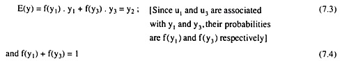
Therefore, when his expected income is y₂, his expected utility would be

E(u) = f(y₁).u₁+f(y₃).u₃ (7.5)

We may now easily prove with the help of Fig. 7.1 that for a person with diminishing MU of income, expected utility E(u) may be less than certain utility u₂, even if his expected income, E(y) = y₂, may be the same as his certain income y₂. In Fig. 7.1, we find that

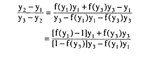
That is, for the chord AC of the curve OE in Fig. 7.1, we obtain

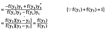
Therefore, the u-coordinate of point B is

Now, when MU of income is diminishing, the curve OE would be concave downwards and so, here, the chord AC would be situated below the curve OE and that is why obtain:

Expected utility, E(u), of expected income, E(y) = y₂, would be less than the certain utility, u₂, of certain income, y₂.

Therefore, we see that if the MU of income of a person be diminishing, then under uncertain conditions, his expected utility [here E(u) = f(y₁).u₁ + f(y₃). u₃] from some amount of expected income (here y₂) would be less than the certain utility of the same amount of certain income. That is why it is said that such a person does not like to take risk and so he is considered to be risk-averse.

In the real world, people generally want to avoid taking risk. That is why they purchase life insurance and health insurance policies and other types of insurance services, and take up the occupations where the wage rates do not fluctuate considerably. We have to remember that a risk-averse person does not like to incur a loss in income.

This is because, for him, MU of income is diminishing and so his total utility from income increases at a diminishing rate as his income rises and, conversely, his TU from income falls at an increasing rate as his income diminishes.

Now we shall speak of those persons who love to enter into risky ventures. In the real world, these risk-lovers are not found frequently, and their psychology is not considered to be normal. We have already proved that a person with diminishing MU of income (as his income rises) is a risk-averter.

We may prove similarly with the help of Fig. 7.2 that, for a person with increasing MU of income, the expected level of utility obtained, under uncertain conditions, from a certain amount of expected income would be larger than the certain amount of utility desired from the same amount of certain income, and that is why such a person loves to take risk. However, two points have to be noted here.

First, since the MU of income of such a person increases as his income increases, his income-utility curve, i.e., OE, would be convex downwards. Second, because of this type of shape of the curve OE, its chord similar to the chord AC of Fig. 7.1 would lie above the curve.

We have to remember here that for such persons a fall in income is not very important. Because, for them, since MU of income is increasing, their TU from income increases at an increasing rate as their income increases and their TU from income diminishes at a diminishing rate as their income decreases.

Finally, we shall speak of those persons who are neither risk-averters nor risk-lovers—they may be called risk-neutrals. These persons remain indifferent between a certain or riskless situation and an uncertain or risky situation, if the expected income in the second situation be equal to the certain income of the first situation.

Here also, like the two cases, we would be able to prove that for persons with constant MU of income, the expected utility under uncertain conditions, of a particular amount of expected income, would be the same as the certain level of utility derived from the same amount of certain income, and that is why they are risk-neutrals.

Here also we have to remember two points. First, the income-utility curve of a person with a constant MU of income would be an upward sloping straight line like the line OE in Fig. 7.3. Second, because of this shape of the line OE, the line segment AC that would be obtained here would lie on the line OE.

We have to note that, for these persons, increases and decreases in income are equally important. Since their MU of income is constant, their total utility of income increases and decreases at the same constant rate as their income increases and decreases.

Risk Premium:

Risk premium is the maximum amount of money that a risk-averse person is ready to forego to avoid taking a risk. In general, the magnitude of the risk premium depends on the risky alternatives that the person faces. In order to explain the point we have reproduced the utility function of Fig. 7.1 in Fig. 7.4. It is clear from the concave downward shape of the curve that the person concerned is a risk-averter.

In Fig. 7.4, let us suppose that the uncertain incomes of the person of y₁ and y₃ have the probabilities that make his E(y) equal to y₂, and the E(U) is obtained from the curve to be By₂. It is seen in the figure that under conditions without risk, the utility of y₂ of income would have been Dy₂ > By₂.

It is also seen in the figure that if the person wanted to have the utility of By₂ = Fy₅ under conditions of certainty, then he would have to accept a ‘certain’ income of y₅ which is less than his E(y) = y₂ by y₂ – y₅. Since in order to avoid taking risk he would accept (y₂ – y₅) less of income, the risk premium here, by definition, would be y₂ – y₅.

Risk Aversion and Income:

The extent of a person’s risk aversion depends on the nature of the risk and the extent of variability of the person’s income. Other things being equal, risk-averse people prefer a smaller variability of their income. We may explain the point again with the help of Fig. 7.4.

Let us suppose that there has been an increase in the variability of his income from what it was previously—now the probable amounts of his income are y₁ and y₄, and not y₁ and y₃, (y₄ > y₃).

Let us also suppose that the probabilities associated with these incomes (i.e., y₁ and y₄) are such that his E(y) remains unchanged at y₂. As a result, his E(u) would be Gy₂ which would be less than his previous E(u) which is By₂. This is because the chord AJ lies below the chord AC.

We have seen, therefore, that if the fluctuations in income is larger, E(u) of income diminishes. Now, if the person concerned wants to have a certain utility of Gy₂ = Hy₆ then the amount of income that he would have to accept is y₆ and this amount is less than his E(y) = y₂ by y₂ – y₆. That is, now the amount of risk premium of the person would be (y₂ – y₆) which would be larger than the risk premium of (y₂ – y₅) that was obtained in the earlier case.

We have seen, therefore, that if the variability of income of a person increases then the amount of his risk premium also increases, i.e., his risk-bearing increases. That is why, a risk- averse person likes to have a smaller variability of income.

Risk Aversion and Indifference Curves:

We may compare the risk aversion of different persons with the help of indifference curves between expected income and risk. The amount of risk-bearing depends upon the variability of income and the measure of this variability is the SD (σ_y).

Therefore, the ICs between expected income and risk would be the ICs between E(y) and σ_y. In Figs. 7.5(a) and 7.5(b), we have shown the ICs of two different persons.

These ICs are sloping upward towards right, since, here, one of the ‘goods’, E(y), is MIB (more-is- better) and the other, σ_y, is MIW (more-is-worse). Consequently, if the risk averter is asked to accept more risk, then in order to remain indifferent he would want to have more of income.

The ICs of the first person in Fig. 7.5(a) are steeper than those of the second person. This gives us that the risk-averseness of the first person is larger than those of the second person.

This is because the rate of increase of E(y) w.r.t. σ_y at any σ_y is larger in the case of the first person than that of the second.