
The below mentioned article provides a complete overview on Break-Even Analysis.
Break-Even Analysis:
Break-even analysis seeks to investigate the interrelationships among a firm’s sales revenue or total turnover, cost, and profits as they relate to alternate levels of output. A profit-maximizing firm’s initial objective is to cover all costs, and thus to reach the break-even point, and make net profit thereafter.
The break-even point refers to the level of output at which total revenue equals total cost. Management is no doubt interested in this level of output. However, it is much more interested in the broad question of what happens to profits (or losses) at various rates of output.
Therefore, the primary objective of using break-even charts as an analytical device is to study the effects of changes in output and sales on total revenue, total cost, and ultimately on total profit. Break-even analysis is a very generalized approach for dealing with a wide variety of questions associated with profit planning and forecasting.
ADVERTISEMENTS:
The following list seeks to highlight some of the more practical applications of break-even analysis:
1. What happens to overall profitability when a new product is introduced?
2. What level of sales is needed to cover all costs and earn, say, Rs. 1, 00,000 profit or a 12% rate of return?
3. What happens to revenues and costs if the price of one of a company’s products is changed?
ADVERTISEMENTS:
4. What happens to overall profitability if a company purchases new capital equipment or incurs higher or lower fixed or variable costs?
5. Between two alternative investments, which one offers the greater margin of profit (safety)?
6. What are the revenue and cost implications of changing the process of production?
7. Should one make, buy, or lease capital equipment?
ADVERTISEMENTS:
Our basic objective here is to introduce the general break-even model, in both graphical and algebraic forms, and to explore the practical use of the model. It may be noted at the outset that although the model has some limitations, if used properly, it can provide management with some valuable guidelines in making certain strategic decisions. After presenting the model these limitations will be brought into focus.
Graphical Presentation of Break-Even Model:
Figure 21.1 presents the simplest and most common graphical representation of break-even analysis. The horizontal axis measures the rate of output, and revenues and costs, measured in rupees, are shown on the vertical axis. Figure 21.1 combines an inverted U-shaped total revenue (TR) curve and the familiar S-shaped short run total cost curve (TC).
The curvilinear shape of the total revenue curve follows from the assumption that the firm faces a downward-sloping demand curve and must reduce its price to be able to sell more. The law of diminishing returns accounts for the curvilinear shape of the total cost curve.
 The vertical distance between TR and TC measures the profit or loss associated with any specific level of output. To the left of Qa and to the right of Qb total costs exceed total revenues, and there are losses.
So there are two break-even points. Between these two points, profits are positive because TR exceeds TC. The point at which profits are maximized (that is, the point at which the vertical distance between TR and TC is the largest) is shown as Qc.
The generalized model in Figure 21.1 is usually simplified to a linear break-even chart, such as that in Figure 21.2. Linearity in the total revenue function implies that the firm is selling in a perfectly competitive market, and hence is a pure price taker and does not have to reduce its price to sell more.
Conversely, linearity in the case of the total cost curve implies that the firm can expand output without changing its variable cost per unit very much. For a relatively narrow output range, this is no doubt a reasonable assumption.
Moreover, we make this linearity assumption to make our analysis simple, and thus to provide management with general profit guidelines, not to suggest exact answers to certain problems. These qualifications apart, there is much to -be said for using the linear break-even model in the real commercial world.

The break-even point is the point where total revenue = total cost, or price per unit = cost per unit. In Figure 21.1 the firm breaks even at two different points B and B’. At both the points there is neither profit nor loss.

In Figure 21.2 the point at which TR equals TC, point QA, is the break-even level of output. To the left of this point the firm incurs losses because TC exceeds TR. But in Figure 21.1 there were two break-even points. In the decision-making process managers often employ a modified breakeven model.
This modification follows from the notion that management may not necessarily think of profit in the economic sense of total revenues, minus total costs. When used for short-run decision making, where a portion of the firm’s monetary resource has already been blocked in the purchase of fixed capital, a more appropriate measure known as the contribution margin or contribution to profit is used.
In the short-run a firm’s initial objective is to cover variable cost. If this cannot be covered, a firm would prefer to close down its operations completely and attempt to minimize its losses. If the price of the product exceeds variable cost, the firm would attempt to expand production with a view to covering fixed cost and make profit subsequently. So output will expand if price exceeds average variable costs.
ADVERTISEMENTS:
The difference between the two (i.e., P — AVC) is called the contribution margin per unit, or average contribution margin. This shows the contribution of the product toward the recovery of fixed cost and toward net profit. If it is multiplied by the sales volume (Q), we arrive at the total contribution margin.
In short, contribution margin refers to the difference between total revenue and total variable cost. For example, if a product sells for Rs. 5 per unit, and overall variable cost is Rs. 3 per unit, each unit sold makes a contribution of Rs. 2 toward the recovery of fixed cost.
Figure 21.3 illustrates a contribution margin break-even chart based on linear cost and revenue curves. Here total net profit TNP, is the difference between TR and TC.
Total contribution margin (or profit) TCM is expressed as:
ADVERTISEMENTS:
TCM = TNP + TFC
TCM = TR – TVC.
Contribution as a Decision Criterion:
The difference between the revenue produced from sale of a product, and its production and selling cost, is the contribution towards fixed costs and to the ultimate net profit. This contribution concept is often used for decision-making purposes.
There is hardly any reason, however, why every product-line made and marketed by the firm should be expected to make the same contribution. By contrast, there is a case for assuming that preference should be given to those product-lines which offer the possibility of making the largest contribution.
An important element of cost-volume-profit analysis is the marginal income ratio or profit-volume ratio, defined as “the percentage of the sales which is available as a contribution to fixed costs and profits after direct costs are deducted.”
ADVERTISEMENTS:
It is expressed as:
![]()
![]()
One may contrast this method with that of ‘full cost’. Suppose that a hypothetical company is considering the relative merits of two products, X and Y.
Initially, it approaches the problem by way of full cost and produces some such statement as the following:

It may apparently seem, from this example, that both products yield the same percentage profit on sales and that there is nothing to choose between them.
ADVERTISEMENTS:
If, however, one focusses on the dubious nature of the cost allocation embodied in the above figures, an alternative presentation might be made on the following lines:

Now we get a completely different picture. Each unit of X sold produces a higher cash contribution and a higher rate of contribution towards fixed costs and profit. It would surely merit the attention of the management in preference to product Y. The relationship is illustrated in Figure 21.4.

In order to adopt this type of approach, one must relate the costs directly to the production and marketing of the product—the costs which could be avoided by not producing the item. Clearly, the selling price must generate sufficient revenue to cover these in the normal course of business.
ADVERTISEMENTS:
If the company is largely a ‘price taker’, having to accept the prevailing market price, the above cost data can be used to determine the product mix which will yield the maximum contribution for the least sales revenue. If, however, the company is a ‘price maker’ with some degree of independence in price fixing, it can use the data as the starting point in price determination.
In a multi-product firm, it is not enough merely to determine the product mix with a view to the maximization of contribution. The firm will be equipped with production facilities, some of which may be specific to given products, whilst others can be used for more than one product, though the demands made on them in terms of time will vary from one product to another.
Thus, in settling for a given pattern of contribution, the manufacturer must make certain that this does not make him suffer from capacity constraints.
As a guide to the solution of this problem it may appear necessary to evolve some yardstick to enable a decision to be made as to which product-line or order is to be discarded, when particular production facilities are overburdened.
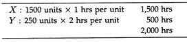
Consider the following example:

The order B contributes Rs. 20,000 to fixed charges and profit as against the Rs. 10,000 provided by order A. But its claim on production facilities if 25 times as great. The result is that the contribution per facility hour is Rs. 200 as against Rs. 250.
ADVERTISEMENTS:
If capacity is inadequate, say 60 hours, to undertake both orders, and if part orders cannot be taken, then the management may be constrained to reject order B. Thus, if the volume of production which the firm can sell exceeds the existing capacity, the optimal results will be obtained by producing those orders which make the maximum contribution per facility hour in the area where the bottleneck occurs.
Example 1:
A company produces two products X and Y. The following facts are given regarding them:


Since the production hour is the limiting factor, product X, which makes greater contribution per hour, will be accorded priority.
Therefore, optimum product mix will be as under:

The remaining 500 hours will be utilised for the production of Y, i.e., 500/2 = 250 units of Y can be produced in the remaining hours.
We know that average net profit, i.e., ANP = P- ATC = P- AVC – AFC or ANP + AFC = P — AVC = ACM or average contribution margin. Now at the break-even point ANP = 0. Therefore, AFC = ACM. So the break-even point can be identified by finding out the level of sales at which AFC = ACM. See Figure 21.5.
Algebra of Break-Even Analysis:
Let us continue to assume linear cost and revenue functions. We may now define the symbols usually used in break-even analysis:


Three Alternatives:
The breakeven point may now be computed in one of three different but interrelated ways:
(1) As a number of units mat must be sold,
(2) Money value of sales, or
(3) As a percentage of plant capacity.
To illustrate, assume that we have a factory that can produce a maximum of 20,000 units of output per month. These 20,000 units can be sold at a price of Rs. 100 per unit. Variable costs are Rs. 20 per unit and the total fixed costs are Rs. 2, 00,000.
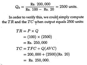
1. By a direct application of Eq. (2) we can compute the number of units that must be sold to break even:
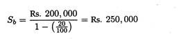
2. If one is to determine the break-even level measured in terms of rupee sales, Eq. (2) has to be slightly modified to yield where Sb denotes the breakeven sales level.
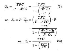
The denominator in equation (3a) provide a measure of the contribution made by the product to recover fixed costs. For our example, the breakeven level in rupee sales is which is the same result that can be obtained by multiplying the break-even quantity by unit price.
In equation (3), the contribution margin is calculated on a per unit basis from the ratio of AVC to price. In equation (3a), the contribution margin is calculated on a total sales revenue basis from the ratio of TVC to TR. The ratio is the same in each case and in both the situations the calculated ratio is subtracted from 1 to yield the percentage of revenue that contributes to recovery of fixed costs or overhead.
3. In order to determine the breakeven point in terms of percentage utilization of plant capacity (%B), (or load factor to be achieved) Eq. (2) has to be modified as follows:
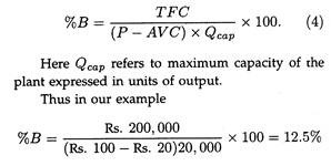
which indicates that the firm can break even by using only 12.5% of its capacity.
Example 2:
Indian Airlines has a capacity to carry a maximum of 10,000 passengers per month from Calcutta to Guwahati at a fare of Rs. 500. Variable costs are Rs. 100 per passenger, and fixed costs are Rs. 3, 00,000 per month. How many passengers should be carried per month to break even? What load factor (i.e., average percentage of seating capacity filled) must be reached to break even?
We may note that P – AVC = Rs. 500 – Rs. 100 = Rs. 400. Then, by equation (7) or (7a) we get

Obtaining Information Necessary for Break-Even Models:
To construct break-even charts or models we have to study a single time period’s income and expense accounts. With the income and expense statements in hand we have to then categorise the various costs as either fixed or variable. We may then proceed to construct our model. The principal advantage of this approach is that it highlights the role of each of the cost categories affecting profits.
Alternatively one can compare a series of income and expense accounts over several time periods in which management has been varying both cost and output levels. This information may then be utilized to arrive at an estimate of an empirical cost function (usually, via regression), which, when combined with the revenue functions, provides information on breakeven levels.
This approach has one obvious advantage that more information is incorporated into the model. But the major problem with this approach is that sufficient data may not be available to enable us to estimate either the cost or revenue functions.
Applications of Break-Even Analysis:
The break-even analysis can throw light on a number of real (commercial) world problems. We may now see how break-even analysis can be used as a tool to assist management in making decisions. We continue to assume that the linear cost and revenue curves are a close enough approximation so as to make the results useful to management.
Adding an MBA Programme:
Suppose the Pro-Vice-Chancellor (Academy) of Calcutta University is contemplating the addition of a special weekend MBA programme for working executives. Two different proposals have been put before the Pro-Vice-Chancellor.
In the first alternative, the university would incur a fixed costs of Rs. 75,000 for microcomputers dedicated to the weekend programme, and experience an average variable cost of Rs. 20 per lecture hour to cover salaries for additional faculty and the incidental incremental expenses associated with it.
In the second alternative, Rs. 50,000 would be spent to raise the capacity of the university’s present mainframe computer, and variable cost per unit is expected to be Rs. 30 per lecture hour.
The P.V.C. is now faced with two specific questions. First, what must the enrolment be for the university to break even with either alternative, if the tuition fee is set at Rs. 70 per lecture hour? Second, how high will the volume (lecture hours) have to be before the profit level of the high investment project equals the profit level of the low investment alternative?
The P.V.C’s first question contains all of the relevant information which can be summarized as follows:
Project 1:
TFC = Rs. 75,000
AVC = Rs. 20 per lecture hour
P = Rs. 70/per lecture hour
Project 2:
TFC = Rs. 50,000
AVC = Rs. 30 per lecture hour
P = Rs. 70 per lecture hour
Substituting these values into Eq. (7) and solving for the break-even volumes (Q1 and Q2, respectively), we get
Q1 = Rs.75, 000/ (Rs.70 – 20)
= 1500 lecture hours
Q2 = Rs.50, 000/ (Rs.70 – 30)
= 1250 lecture hours.
Thus the first project would appear to be riskier because it has higher fixed costs and higher breakeven level. That is, it requires a larger number of lecture hours to cover all of its costs. On the contrary, the contribution margin on a per-unit basis from the project is Rs. 50 per lecture hour versus only Rs. 40 for the second project.
The P.V.C.’s second request was to determine the output level at which the profit from the first project equals that of the second project. This becomes a crucial issue because the second project can break even at 1250 hours and earn a profit of Rs. 10,000 at 1500 hours, whereas the second project must reach 1500 hours before breaking even.
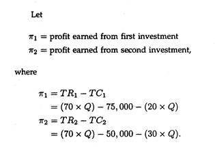
To find the volume level at which π1 equals π2, we simply set Eq. (16) and (17) equal to each other and then solve for Q:
50Q = 75,000 = 40Q – 50,000
10Q = 25,000
Q = 2500 lecture hours.
Output will have to reach 2500 lecture hours for project 1 to be as profitable as project 2. Beyond 2500 hours, the comparative profitability of project 1 becomes greater because of the greater contribution per unit. Conversely, below 2500 hours, project 2 becomes preferable. With this information, the P.V.C. might be interested in estimating the likely number of lecture hours to be generated by the new MBA programme.
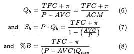
Break-Even Models and Planning for Profit:
The break-even point represents the volume of sales at which revenues equal expenses; that is, at which profit is zero. Computationally, the breakeven volume is arrived at by dividing fixed costs (costs that do not vary with output) by the contribution margin per unit, i.e., selling price minus variable costs (costs that vary directly with output).
In certain situations, and especially in the consideration of multi-products, break-even volume is measured in terms of rupee sales value rather than units.
This is done by dividing the fixed costs or overheads by the contribution margin-ratio (contribution margin divided by selling price). Generally, in these types of computations, the desired profit is added to the fixed costs in the numerator in order to ascertain the sales volume necessary for producing the target profit.
If management plans for a certain profit, then revenues needed to cover all costs plus the desired profit is
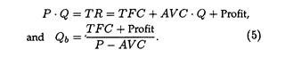
This information can be shown graphically, as in Figure 21.6. In this example, fixed costs are Rs. 1, 00, 000 and variable costs are Rs. 12.50 per unit. The price charged is Rs. 25.00 per unit and the breakeven point occurs at 8,000 units of production (verify this using the formula). If management wants a profit of Rs. 50,000, they will have to produce and sell 12,000 units (again, you should verify this).

To sum up, a break-even point can be found by calculating all fixed costs for a period, calculating the variable costs per unit, adding the fixed and variable costs, and deciding on the price of the product or service (or income per unit).
It can be used for multi- product situations if the product mix is constant and if separate revenues and costs can be developed for each product, although this usually presents a problem since separating these costs is no doubt difficult in practice.
Instead of focusing exclusively on the breakeven level of output, management may at times be interested in estimating the volume (QT) needed to earn enough not only to cover all costs but earn a’’ target “(PRT).
If this is the objective, the break- even equations have to be modified as follows:
To illustrate this process, we go back to the example used in our discussion of the linear breakeven model.
The necessary information is given below:
Qcap = 2000,
P = Rs.100,
AVC = Rs.20,
TFC = Rs.200, 000
Qb = 2500 units,
Sb = Rs.250, 000,
%B = 12.5.
Now suppose that management wants to earn a target profit of Rs. 50,000. Making the appropriate substitution into Eqns. (6) through (8) we obtain the new levels of Qb = 321,500 and %B = 15,625. If we add this target profit to the fixed costs we see that the break-even levels of all three factors get increased.
The information in this example could be extended so as to make provisions for such factors as payment of taxes or for payment of any other fixed obligations that might be associated with the fixed costs (such as interest payments on bonds or debentures used to finance an investment).
Example 3:
Suppose the objective of Indian Airlines is to make a profit of Rs. 2, 00,000 per month. The question is: how many passengers should be carried per month to reach the profit target? One final question is: What is the maximum amount of profit that can be made by Indian Airlines?
Now to answer to first question we can use the following expression:


which is the maximum amount of profit that can be earned by Indian Airlines by fully utilizing its capacity (i.e., by 10,000 passengers per month).
Example 4:
To illustrate the case of break-even analysis with taxation, suppose that r represents the tax rate percentage, PAT is profits after taxes, and PBT is profits before taxes. The relationship between PAT and PBT can be shown to be
PAT = (1 – r) PBT (9)
Or, PBT = PAT (1-r) (10)
Consider the case when the tax rate is 50%. An after-tax profit of Rs. 50,000 would require a before- tax profit of
PBT= Rs.50, 000 / (1-0-5) = 100,000
This figure of Rs. 1, 00,000 would then be introduced into the numerator of the break-even ratio, as was done in Eq. (6) through Eq. (8). Essentially, the introduction of taxes or other fixed obligations will result in increasing the break-even levels of output in numbers, rupees sales, and capacity.
Break-Even Chart Alternatives:
The break-even quantity is not a fixed number. Management can alter the quantity by changing the controllable variables. Since plant capacity is limited in the short run, profits can be increased only by shifting the break-even point to a lower level of production or sales which can be accomplished by manipulating three variables: fixed costs, variable costs, or price. Herein lies an important application of break-even charts in profit planning, control, and forecasting.
To illustrate this situation, suppose that we have collected the following information (all tabulated on a per month basis):

Figure 21.7 depicts the effect of manipulating the three variables on the break-even level of output. Panel (a) illustrates the original situation where the break-even level of output is 100 units and total revenue and cost equal Rs. 1,500. Panel (b) depicts the impact of reducing fixed costs from Rs. 600 to Rs. 200.
The shaded portion on the graph provides a measure of the original profits, and the crosshatched area provides a measure of the increase of profits.

If the fixed costs can be reduced to Rs. 200, the breakeven level of output can be brought down to approximately 33 units, and break-even costs and revenues to approximately Rs. 497. The impact of reducing variable costs to Rs. 5 is shown in panel (c).
In this situation, costs and revenue both fall to Rs. 900 and the break-even output level of 60 units is reached. Panel (d) presents the final option of increasing the market price of the product to Rs. 17 per unit.
When the price is increased, the slope of the total revenue curve changes, while the break-even level of output falls to 75 units. A comparison of the three alternative methods of altering the break-even quantity indicates that the most promising, in terms of profitability, is the case where the fixed costs are reduced to Rs. 200.
Example 5:
Suppose you have the following information about a hypothetical company:
Plant capacity =100 units
AVC = Rs.7per unit
P = Rs.12 per unit
TFC = Rs.400
Qb = 80 units
TR (at capacity) = Rs.1,200
TC (at capacity) = Rs.1, 100
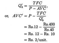
Suggest alternative ways of reducing the breakeven quantity by 50%.
There are three ways of reducing the break-even quantity:
(a) Reducing total fixed cost,
(b) Reducing total variable cost and
(c) Raising product price,
(a) In the example, if total fixed cost is reduced to Rs. 200, we can reduce the break-even quantity to 40, or
![]()
(b) Alternatively, reduction of the break-even quantity to 40 may be achieved by a reduction in AVC. Thus
Thus a 50% reduction in break-even quantity requires more than 70% reduction in total variable cost (from Rs. 7 to Rs. 2).
(c) Finally, the price of the product may be raised to achieve the new break-even quantity thus:
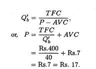
It may be noted that with an increase in price, a decrease in sales might be expected, but even with reduced sales, a sizable increase in profit could result.
The Margin of Safety (Profit):
So long only one of the controllable variables (price, or fixed or variable costs) was changed, but in practice management may have the power to change all three of them simultaneously. In order to be able to assess the impact of changing more than one of the variables we often adopt a modified version of break-even analysis.
This modification looks at the ratio of total net profit to total fixed cost. By focussing on this ratio, we are virtually focussing on the margin of profit that the firm is currently making, and the losses it would incur in case sales fall below the break-even level.
The larger the ratio of profits to total fixed costs, the better it is for the firm (from the standpoint of safety). Hence this ratio is called the margin of safety or the margin of profit.
The margin of safety can be expressed as:

where Qs refers to the number of units actually sold.
Example 6:
We may now illustrate the application of the margin of safety in performing the marketing function, and we suppose that we have the following information:

The production manager has suggested a change in a production technique that will increase variable costs by Rs. 5 per unit. The new item will sell for Rs. 15 less than the old one and the marketing manager estimates that this price reduction will increase sales to 775 units.
However, he also suggests that Rs. 10,000 will have to be spent on advertising to inform potential customers of the price reduction.
Management has now to decide which of four alternatives is to be preferred:
(1) Maintaining the status quo,
(2) Adopting the production technique, reducing price and undertaking the advertising campaign ,
(3) Maintaining profits without undertaking the advertising programme, and
(4) Not reducing the selling price but conducting the advertising programme. The computations for these four alternative are presented below:
1. Maintain status quo:

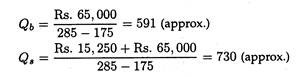
2. Undertake all of the options:
Suppose the new production technique is adopted; variable costs increase to Rs. 175 per unit; price is reduced to Rs. 285 and sales increase to 775 units; and Rs. 5,000 is spent on advertising:

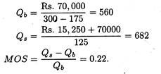
3. If the same level of sales is maintained as in option 2 but without the advertising programme, we have the following results:
It is to be noted that the projected sales are lower here than with the second option because of not undertaking the advertising programme.
![]()
4. If the same level of profit as in option 2 is maintained but price is not lowered and the advertising programme is undertaken, we have the following results:
Example 7:
Suppose a company produces three-wheelers for sale to commercial users at Rs. 35,000 each. The plant is currently operating at 60% of its capacity of 80 units per year, at a total fixed cost of Rs. 6, 00,000 and an average variable cost of Rs. 20,000 per unit.
The firm is contemplating a change in product design that will increase the average variable costs by Rs. 1,000. Also an advertising campaign will be launched at a cost of Rs. 1, 20,000, to announce that the new improved model will sell for Rs. 2,000 less than the old one.
The marketing manager estimates that these measures will increase sales to 90% of plant capacity. Assuming that the marketing manager is correct, what will be the effects of all these changes on the break-even sales volumes and on annual profits?
Solution:
In the existing situation the break-even sales volume is


The margin of safety clearly indicates that the third option is preferable. The implication of this higher margin of safety is that management can undertake this option with the knowledge that it can come closer to incurring its fixed costs even if the expected level of sales fails to materialize.
Applications of Break-Even Charts:
Comparison of Different Production Techniques:
One of the primary tasks of the production manager is to make decisions such that production costs are minimized. Break-even analysis can be fruitfully utilized by management in making cost comparisons among production techniques that involve different fixed and variable cost structures.
As a general rule, more capital-intensive methods involve a cost structure with greater fixed and lower variable costs. By contrast, labour-intensive production techniques usually imply lower fixed and higher variable costs. Thus the cost advantage of each of these two production techniques depends on the level of output.
In most production processes it is observed that the higher the level of output, the more efficient will be the capital-intensive technique, and the lower the level of projected output the more efficient will be the labour-intensive technique.
This point may now be illustrated.
Suppose that the production analyst has derived the following two cost functions for different production techniques:
TCa = Rs. 170 + Rs. 1.40Q
TCb = Rs.520 + Rs. 0.85Q.
Technique (a) is the labour-intensive production method and technique (b) is the capital-intensive method.
The first step in this type of practical situation is to determine the level of output at which the two production techniques are equally efficient. To do this, we simply set the total cost functions equal to each other and solve for Q as follows:
TCa = TCb
Rs. 170 + 1.40Q = Rs. 520 + Rs. 0.85Q
Rs. 1.40Q- Re. 0.85Q = Rs. 520- Rs. 170
or, Q — 636 (approx.).
For any output level which is less than 636 units, production technique (a) is more efficient, and for any output level above this initial quantity, production technique (b) will involve a lower cost.
If this type of information in available, the production analyst may contact the marketing manager about the projected level of sales. The marketing manager suggests that the most probable level of sales is 700 units with deviation of 250 units and that the distribution of sales is approximately a normal distribution.
This information may now be summarized in one graph shown is Figure 21.8. Now the pertinent question faced by the production analyst is this: What is the probability of sales equalling or exceeding the break-even level of 636 units? This corresponds to the shaded area under the normal probability curve as shown in Figure 21.8.

To arrive at the correct answer to the question, the first step is to compute the appropriate Z value as follows:

The appropriate percentage of the normal probability curve that corresponds to this Z value is given in any standard textbook of statistics. Corresponding to the Z value of 0.26 is the entry 0.1026.
Because 50% of area of the normal curve lies to the right of the mean, the shaded area equals 60.26% (obtained by summing 50% and 10.26%). With this information, the production manager can now bring the information to the notice of top management that there is approximately a 60% probability that the capital-intensive plant will lead to a lower cost per unit.
We can use exactly the same type of approach to evaluate such questions as the following:
Should we buy or lease a piece of equipment?
Should we make or buy a part?
Should the plant size be expanded?
The Degree of Operating Leverage:
Linear cost-volume-profit analysis can also be used for analysing the financial characteristics of difficult production processes. By using linear breakeven charts we can ascertain how total costs and profits vary with output as the firm uses more and more capital-intensive methods of production, and thus raising the proportion of fixed costs and reducing that of variable costs.
Operating leverage “reflects that extent to which fixed production facilities, as opposed to variable production facilities, are used in operations.” The relation between operating leverage and profit variation is shown if Figure 21.9, in which we compare three firms, X, Y, and Z each having a differing degree of leverage. The fixed costs of operations in Firm Y are considered to be the most representative of all.
It uses equipment with which one operator can turn out a few or many units at the same labour cost, to about the same extent as the average firm in the industry. Firm X uses less capital equipment in its production process and has lower fixed costs.
But X’s variable cost increases more sharply than that of Y. Firm X breaks even at a lower operation cost than does Firm Y. In Figure 21.9, at a production level of 40,000 units, Y is losing Rs. 8,000, but X breaks even.
Here firm Z is having the highest fixed costs because its uses modern, sophisticated and hence costly machines that require very little labour per unit of output. With such an operation, its variable costs rise very slowly.
Because of the high overhead resulting from charges associated with the expensive machinery, Z’s break-even point is higher than that of either X or Y. Once firm Z reaches its breakeven point, however, its profits rise faster than do those of X and Y.
The degree of operating leverage has been defined as the percentage change in profit that results from a 1 per cent change in units sold. It shows how a given change in volume affects profits.
This may be precisely expressed as:

where π is profit and Q is the quantity of output in units.
Since the degree of operating leverage is a ratio of two percentage changes, it is not fundamentally different from an elasticity concept. It has been called by Pappas the operating leverage elasticity of profits. In case of linear cost and revenue curves, this elasticity measure will vary depending on the particular part of the breakeven chart that is under consideration.
For instance, the degree of operating leverage is always very close to the break-even point, where a very small change in sales volume can produce a very large percentage increase in profits, simply because the base profits are close to zero near the break-even point.


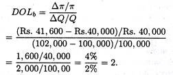
For firm Y, in Figure 21.9(b) the degree of operating leverage at 100,000 units of output is 2.0. This is calculated as follows:

We arbitrarily assume that the change in Q (∆Q) = 2,000. If we assume any other ∆Q, for example, ∆Q = 1,000 or ∆Q = 4,000 the degree of operating leverage will still turn out to be 2, because we continue to use linear cost and revenue curves. But if we choose a base different from 100,000 units, the degree of operating leverage (DOL) will be found to be different from 2.
For linear revenue and cost relations, it is possible to calculate the degree of operating leverage for any level of output Q: The change in output is defined as ∆Q. Fixed costs are held constant so the change in profit is ∆Q(P — AVC). where all the terms have their usual meanings.
The initial level of profit is Q (P – AVC) – TFC, and the percentage change in it is:
![]()
The percentage change in output is ∆Q/Q, so the ratio of the percentage change in profits to the percentage change in output may be expressed as:
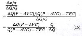
A little manipulation will yield the following
![]()
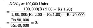
Using Equation (16), we find Y’s degree of operating leverage at 1,00,000 units of output to be:
Equation (16) can also be applied to firms X and Z. If this is done, X’s degree of operating leverage at 100,000 units become 1.67; Z’s is 2.5. Thus with a 10 per cent increase in volume, Z (the firm with the most operating leverage) will experience a profit increase of 25 percent. For the same 10 percent sales gain, X the firm with the least leverage, will experience only a 1.67 percent profit gain.
The calculation of the degree of operating leverage through equation (13) and (16) shows the same thing that Figure 21.8 shows graphically; that the profits of firm Z, the company with the most operating leverage, is most responsive to changes in sales volume, while those of firm X, which has only a small amount of operating leverage, is relatively less responsive to volume changes.
Firm Y, with an intermediate degree of leverage, lies in-between the two extreme situations.
Evaluation of Break-Even Models:
Break-even models are relatively simple to construct and to interpret by both analysts and management. Furthermore, they are inexpensive, especially when compared to more complex models and, given their widespread applicability, they confer significant cost advantages.
In general, the data needed to apply break-even analysis are readily available, and the cost of such data collection is nominal. However, break-even analysis is not free from defects. It is subject to abuse and misinterpretation.
So one who applies this technique of profit planning must be aware of the following limitations and qualifications associated with break-even models:
1. Prima facie, since most of the data utilized to construct break-even charts and models are derived from accounting records and statements, financial analysts must be aware of the limitations of accounting data.
In particular, as Bails and Peppers have cautioned that “the cost estimates and functions must be adjusted to consider implicit costs, depreciation estimates, and inappropriate assignment of overhead costs. This is, one must ensure that the measures of total cost represent only those costs that are incurred as a result of the decision being considered, and that it does not include costs that will be incurred by the firm regardless of the decision made about the problem at hand”.
2. Secondly, so far we have focused on linear applications of the break-even model. However, the same analysis could be extended with curvilinear cost and revenue functions. But in such cases we get two break-event points, not one. True enough, linear cost-volume-profit analysis is very weak with regard to costs.
The linear relations indicated by the chart do not hold at all output levels. With increase in sales, existing plant and equipment are worked beyond capacity, thus reducing their productivity. This situation results in a need for additional workers and frequently longer working days, which may require the payment of overtime wages.
All these factors cause variable costs to rise very sharply. Additional plant and equipment may be required, increasing fixed costs. Furthermore, over an extended period of time the products sold by the firm change in quality and quantity. Such changes in optimum product mix influence both the level and the slope of the cost function.
3. Thirdly, the assignment of selling and marketing costs can be difficult and may require some sort of subjective decision making. This follows from the fact that the relationship between output and selling costs is a one-sided one. Moreover, there is hardly anything to indicate that the relationship between output and marketing costs is particularly stable over time or over various output ranges.
4. Moreover, we implicitly assumed so far that the firm was concerned with only one product. But in practice we observed that most firms are multi-product firms. The most common approach for a heterogeneous product mix is to measure output in terms of rupee sales volume. However, this approach does not completely overcome the problems associated with multiple products.
5. Linear cost-volume-profit analysis is especially weak in what it implies about the sales possibilities for the firm. Any given linear-cost-volume profit chart is based on a fixed selling price. Therefore, with a view to studying profit possibilities under alternative prices, a whole series of charts is necessary, one chart for each price. Non-linear cost-volume-profit analysis can be used as a preferable alternative.
6. There are several other problems with breakeven analysis, however, which usually mean it can only provide a rough approximation for planning decisions:
(a) Usually, the cost and revenue calculations are much more complex than the simple examples used here. Often managers do not know what these fixed and variable costs are.
(b) It is difficult, if not impossible, to estimate what sales will be at various price levels, or to accurately project total revenues.
(c) Materials and other variable costs may fluctuate widely. Like prices, they are not constant over time. Similarly, it is not clear which fixed costs (like overhead costs) should be included. For example, what part of the president’s salary is to be included for a given product?
A considerable amount of judgement is required to classify the expenses as either fixed or variable. If fixed expenses are overstated, the break-even point is overstated, which could lead to missed opportunities since that sales level is considered unattainable.
If fixed expenses are understated, the break-even point is understated, which could lead to a commitment of resources to attain an undesirable level of sales. If variable expenses are overstated, fixed expenses are understated (and vice-versa) leading to the two preceding situations.
7. In fact, cost behaviour is the response of cost to a variety of influences. Therefore, when working out a cost-volume-profit analysis, we must take into account any factor which may have an effect on the results, and realize that the breakeven graph is only a pictorial expression which relates costs and profit to activity. The graph tends to over-simplify the real situation as there are other effects besides sales volume.
(a) Cost and revenues are shown as straight lines. But in practice, selling prices do not necessarily remain fixed, and the revenue may change depending on the quantities of goods sold directly, sold through agents and sold at a discount. The slope of the graph will not be constant in practice. It will vary under different circumstances.
(b) Variable costs may not be proportional to volume for various reasons such as overtime working, reductions in the price of materials when bulk discounts are negotiated, or because of an increase in price of materials when demand outstrips supply. If sales are made over a wider area, marketing costs tend to increase sharply.
(c) Fixed costs do not always remain constant during the period of activity.
(d) The efficiency of production or a change in production methods is likely to have an effect on variable costs.
(e) The various quantities of different goods sold (the sales mix) may not change the total sales value considerably but they may change the quantum of profit depending on the proportion of low and high-margin goods sold.
For these reasons, break-even analysis is a critical planning tool that can provide a manager with useful insights about the dynamic relationships among expenses, volumes and profits. But, like other planning techniques, it must be used with care with a view to avoiding the risk of making inappropriate decisions.
Implications for Managers:
For organizations that are concerned with profits or costs, financial planning techniques are the basis for all other tactical planning. Break-even analysis is at the heart of most tactical planning. One firm was actually selling every item it produced at a loss because it did not go through this exercise. The losses on this product were covered by profits on other lines.
Later, when a break-even analysis was done, the situation was rapidly (and profitably) corrected. In practice, you will have some problems in classifying costs as fixed or variable, or even in assigning them to a specific product. Again, making the attempt will uncover problems and opportunities and give you planning insights you didn’t have before.