Short-run and Long-run Supply Curves (Explained With Diagram)

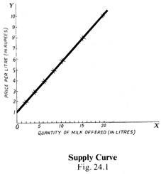
In the Fig. 24.1, we have given the supply curve of an individual seller or a firm. But the market price is not determined by the supply of an individual seller.

Rather, it is determined by the aggregate supply, i.e., the supply offered by all the sellers (or firms) put together.

This is the supply of the whole industry. Thus, the supply curve of an industry depicts the various quantities of the product offered for sale by the industry at various prices at a given time.

The quantities that the industry may offer to sell will depend on the price of its product in relation to the cost conditions of the firms. The cost conditions, in turn, depend on the prices of the factors of production or inputs used by the firms.

Short-run Supply Curve:

By ‘short-run’ is meant a period of time in which the size of the plant and machinery is fixed, and the increased demand for the commodity is met only by an intensive use of the given plant, i.e., by increasing the amount of the variable factors.

Under perfect competition, a firm produces an output at which marginal cost equals! Price. If the price is higher than the marginal cost, it will pay the firm to expand its output so as to equal its price. If, on the other hand, the price is less than the marginal cost, it is incurring a loss, and it will reduce its output till the marginal cost and the price are made equal. Hence, the marginal cost curve of the firm is the supply curve of the perfectly competitive firm in the short-run.

But, even in the short-run, a firm will not supply at a price below its minimum average variable cost. That is, in the short-run, a firm must try to cover its’ Variable cost at least. Hence, the short-run supply curve of a firm coincides with that portion of the short-run marginal cost curve which lies above the minimum point of the short-run average variable cost (SAVC) curve.

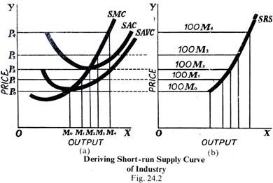
The following diagram [Fig. 24.2(a)) will make it clear:

In this diagram, Fig. 24.2(a) relates to a firm and 24.2(b) gives the supply curve of the industry. First look at the Fig. 24.2(a), which relates to a single firm. Along the axis OX are represented the output supplied and along OY the prices. SMC curve is the short-run marginal cost curve, and, as mentioned above, it is the short-run supply curve of the firm. But only that portion of SMC curve which lies above the short-run average variable cost (SAVC), which means the thick portion above the dotted portion.

Thus, at the price OP₀, OM₀ output will be supplied, at OP₁ price, OM₁, quantity will be supplied at OP₂ price, OM₂ will be supplied, and so on. Nothing will be supplied below the price OP”, because prices below OP₀ correspond to the dotted portion of the SMC which is below the minimum point of the SAVC (short-run average variable cost) curve.

Now from the supply curve of a firm, let us derive the supply curve of the “entire” industry of which all the firms are a constituent par) The supply curve SRS of the industry “‘is derived by the lateral summation (i.e., adding up sideways) of that part of all the firms’ marginal cost curves which lies above the minimum point on their average friable cost curves. This industry is supposed to consist of 100 identical firms like the firm represented by the Fig. 24.2(a).

It can be seen that at OP„ price, 100 OM₁ are supplied, at OP, price 100 OM , are supplied, at OP, price 100 OM, are supplied, and so on. We see that the short-run supply curve SRC of the industry rises upwards, because the short-run marginal curve SMC rises upwards.

Long-run Supply Curve:

The long-run is supposed to be a period sufficiently long to allow changes to be made both in the size of the plant and in the number of firms in the industry. Whereas in the short period, an increase in demand is met by over-using the existing plant, in the long-run, it will be met not only by the expansion of the plants of the existing firms but also by the entry into the industry of new firms.

Moreover, we have seen that, in the short-run, a firm produces that output at which its marginal cost is equal to the price. But, in the long-run, the price must be equal to both the-marginal cost and the average cost. The reason is that an industry will be in equilibrium when all firms in the industry are making normal profits, and they will be making normal profits only if the price, i.e., average revenue (AR) is equal to average cost AC.

The shape of supply curve, in the long run, will depend on whether the industry is subject to the law of constant return (i.e., constant costs), or to diminishing returns (i.e., increasing costs) or to increasing returns (i.e., dimin­ishing costs). We show these curves below.

Supply Curve of Constant Cost Industry:

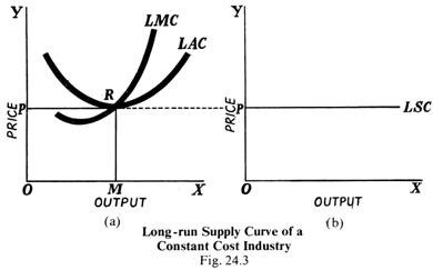
The supply curve of the constant cost industry is shown in the following diagram (Fig. 24.3).

In the Fig. 24.3(a) which relates to a firm, LMC is the long-run marginal cost curve, and LAC is the long-run average cost curve. They intersect at R which means that at the point R, the marginal cost is equal to the average cost. Here they are also equal to price OP. The output at this point is OM. Thus, at the output OM, MC = AC = Price.

Now look at the Fig. 24.3(b). Corresponding to OP price, the long-run supply curve is LSC, which is a horizontal straight line parallel to the X-axis. This means that whatever the output along the X-axis, price is the same OP where the marginal cost and average cost are equal. The cost remains the same, because it is a constant cost industry.

It is an industry in which, even if the output is increased (or decreased), the economies and diseconomies cancel out so that the cost of production does not change. Also, when new firms enter the industry to meet the increased demand, they do not raise or lower the cost per unit.

Thus, the industry is able to supply any amount of the commodity at the price OP which is equal to the minimum long-run average cost which ensures normal profit to all the firms engaged in the industry. That is, every firm will be in the long-run equilibrium where Price = MC = AC. All firms have identical cost conditions.

Hence, in the case of a constant cost industry, the long-run supply curve LSC is a horizontal straight line (i.e., perfectly elastic) at the price OP, which is equal to the minimum average cost. This means that whatever the output supplied, the price would remain the same.

Supply Curve of an Increasing Cost Industry:

In the case of an increasing cost industry, the cost of production increases as the existing firms expand or the new firms enter into the industry to meet an increase in demand. The external diseconomies outweigh the external economies. The increased demand for the productive resources required to produce larger output to meet increased demand for the product raises their prices resulting in higher cost of production.

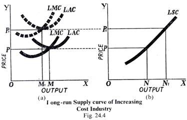
The rise in costs will shift both the average and marginal cost curves upward and the minimum average cost will rise. This means that the additional supplies of the product will be forthcoming at higher prices, whether the additional supplies come from the expansion of the existing firms or from the new firms which may have entered the industry. All this is shown in the following diagram (Fig. 24.4).

The Fig. 24.4(a) shows the position of individual firms. The position of the dotted LMC and LAC curves shows that they have been shifted upwards where each firm achieves a long-run equilibrium so that the price OP, =MC = AC. But, in the Fig. 24.4(b) which relates to the industry, we find that at the price OP i larger amount ON₁ is supplied than at the price OP (i.e., ON).

This means that the long-run supply curve LSC slopes upwards to the right as the output supplied increases. That is, more will be supplied at higher prices. This is probably typical of the actual competitive world, because higher prices have to be paid for the scarce productive resources to attract them from other uses so that production in this particular industry may be increased. Thus, we see that in the case of an increasing cost industry, the long-run supply curve slopes upward to the right.

Supply Curve of a Decreasing Cost Industry:

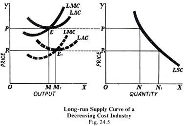
In a decreasing cost industry, costs decrease as output is increased either by the expansion of the existing firms or by the entry of new firms. In this case, the economies of scale out-weight the diseconomies, if any. This happens when a young industry grows in a new territory where the supply of productive resources is plentiful. The net external economies will push the cost curves down so that the additional supplies of the output are forthcoming at lower prices.

The following diagram (Fig. 24.5) makes the whole thing clear:

The Fig. 24.5(a) shows how the new, i.e., dotted LMC and LAC curves have been shifted downwards from their original position, when the LMC and LAC curves intersect at E where every firm was the equilibrium and was producing OM. The new curves intersect at E₁ which means that, at this point, the firms in the industry have achieved the- long-run equilibrium, each producing OM, output, so-that the price OP =MC = AC. But looking at the Fig. 24.5(b), we find that, at OP₁ price, ON is supplied which is more than ON supplied at the original price OP.

The LSC slopes downwards to the right which means that the additional supplies of the output are forthcoming at lower prices, since both the marginal cost and average cost have fallen owing to cheaper supplies of the productive resources.

Summing Up:

Thus, we find that, while the short-run supply curve of the industry always slopes upwards to the right, the long-run supply curve may be a horizontal straight line, sloping upwards or sloping downwards depending upon the fact whether the industry in question is a constant cost industry, increasing cost industry or decreasing cost industry. But the long-run upward sloping curve is more typical of the actual world.